Mac OS X

2022-07-21 18:37

Comments

Here are some notes about how I configure Mac OS X.

Docker

2020-11-30 18:37

Comments

Some notes about using Docker to host various applications like Heptapod, Discourse, CoCalc etc. on Linux and AWS.

super_hydro: Superfluid Hydrodynamics Explorer

2020-06-01 12:00

Comments

highlight

Vortices in a rotating BEC with a pinning site and tracer particles.

super_hydro: Exploring Superfluids¶

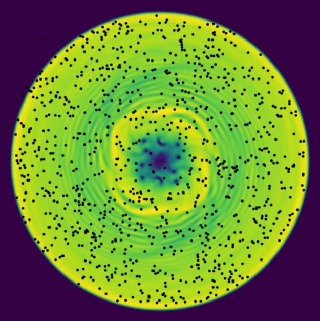
Nobel laureate Richard Feynman said: "I think I can safely say that nobody really understands quantum mechanics". Part of the reason is that quantum mechanics describes physical processes in a regime that is far removed from our every-day experience – namely, when particles are extremely cold and move so slowly that they behave more like waves than like particles.

This application attempts to help you develop an intuition for quantum behavior by exploiting the property that collections of extremely cold atoms behave as a fluid – a superfluid – whose dynamics can be explored in real-time. By allowing you to interact and play with simulations of these superfluids, we hope you will have fun and develop an intuition for some of the new features present in quantum systems, taking one step closer to developing an intuitive understanding of quantum mechanics.

Beyond developing an intuition for quantum mechanics, this project provides an extensible and general framework for running interactive simulations capable of sufficiently high frame-rates for real-time interactions using high-performance computing techniques such as GPU acceleration. The framework is easily extended to any application whose main interface is through a 2D density plot - including many fluid dynamical simulations.

Javascript

2020-01-25 08:18

Comments

JavaScript¶

This post discusses JavaScript.

Prerequisites: Models

2020-01-06 23:58

Comments

Eli Francis

Prerequisites: Models¶

This post describes various models that are useful for demonstrating interesting physics.

Bayesian Analysis

2019-11-06 21:15

Comments

Bayesian Analysis¶

In this post we perform a simple but explicit analysis of a curve fitting using Bayesian techniques.

kyle-elsasser

2019-10-31 23:23

Comments

Kyle Elsasser

Kyle Elsasser¶

Kyle was raised on a farm in the mountains of northern Idaho before becoming a Nuclear Reactor Technician on US Navy submarines and later a firefigher/EMT back in his hometown. His curiosity got the better of him and he attended Eastern Washington University, completing a bachelor's degree in Physics and one in Mathematics in 2017 before continuing to Washington State University to pursue his PhD in Physics.

Currently, he is working jointly under Dr Forbes and Dr Bose to re-derive the Tolman-Oppenheimer-Volkoff (TOV) equations for arbitrary rotation speeds, and has interest in investigating the mechanisms that cause neutron star glitching.

chunde-huang

2019-10-30 23:23

Comments

Chunde Huang

Chunde Huang¶

Chunde comes from China where he got his bachelor degree (Software Engineering) and master degree (Computer Science) from Xiamen University, his major research was computer vision and machine learning. He worked as a professional software engineer for three years with experience on embed system framework development (C++ middleware for Android OS), smart traffic surveillance (object detection and tracking) and distribute system (Content Distribution Network). He started his pursuit of Ph. D in physics in 2013 at WSU.

praveer-tiwari

2019-10-30 23:23

Comments

Praveer Tiwari

Praveer Tiwari¶

Praveer comes from India where he got his BSc-MSc(Research) degree(Physics) from Indian Institute of Science, his major research was on Accretion Disk Modeling and Gravitational Wave Data Analysis. He started his pursuit of Ph.D in physics in 2016 at WSU. Since 2017, he worked in professor Jeffrey McMahon Group learning different aspects of machine learning and computational condensed matter.

Currently, he is working jointly under Dr Forbes and Dr Bose. He is working on constraining the parameters of the equation of state of neutron stars using the gravitation wave detection. He is also working on employing novel machine learning techniques to characterize different aspects of gravitational wave detections.

Errata

2019-02-19 02:58

Comments

Nathan Dumlao

Errata¶

This post collects various typos etc. in my publications. If you think you see something wrong that is not listed here, please let me know so I can correct it or include it.

Matplotlib subplots and gridspec

2019-02-05 13:04

Comments

Matplotlib Subplot Placement¶

Here we describe how to local subplots in matplotlib.

In [ ]:

import sys
sys.exec_prefix

Overview¶

We start with several figure components that we would like to arrange.

In [1]:

%pylab inline --no-import-all

def fig1():
    x = np.linspace(0, 1, 100)
    y = x**2
    plt.plot(x, y)
    plt.xlabel('x'); plt.ylabel('x^2')
    
def fig2():
    x = np.linspace(-1, 1, 100)
    y = x**3
    plt.plot(x, y)
    plt.xlabel('x'); plt.ylabel('x^3')

Populating the interactive namespace from numpy and matplotlib

Here is a typical way of arranging the plots using subplots:

In [12]:

In [13]:

def fig3():
    plt.subplot(121)
    fig1()
    plt.subplot(122)
    fig2()
fig3()

Now, what if we want to locate this composite figure? GridSpec is a good way to start. It allows you to generate a SubplotSpec which can be used to locate the components. We first need to update our previous figure-drawing components to draw-themselves in a SubplotSpec. We can reuse our previous functions (which use top-level plt. functions) if we set the active axis.

In [24]:

from functools import partial
import matplotlib.gridspec
import matplotlib as mpl

def fig3(subplot_spec=None):
    if subplot_spec is None:
        GridSpec = mpl.gridspec.GridSpec
    else:
        GridSpec = partial(mpl.gridspec.GridSpecFromSubplotSpec, 
                           subplot_spec=subplot_spec)
    gs = GridSpec(1, 2)
    ax = plt.subplot(gs[0, 0])
    fig1()
    ax = plt.subplot(gs[0, 1])
    fig2()
fig3()

In [26]:

fig3()

In [25]:

fig = plt.figure(constrained_layout=True)
gs = GridSpec(2, 2, figure=fig)
fig3(subplot_spec=gs[0, 0])
fig3(subplot_spec=gs[1, 1])

Inset Axes¶

If you want to locate an axis precisely, you can use inset_axes. You can control the location by specifying the transform:

bbox_transform=ax.transAxes: Coordinates will be relative to the parent axis.
bbox_transform=ax.transData: Coordinates will be relative to the data points in the parent axis.
bbox_transform=blended_transform_factory(ax.DataAxes, ax.transAxes): Data coordinates for $x$ and axis coordinates in $y$.

Once this is done, locate the axis by specifying the bounding box and then the location relative to this:

bbox_t_anchor=(left, bottom, width, height): Bounding box in the specified coordinate system.
loc: Location such as lower left or center.

In [64]:

from matplotlib.transforms import blended_transform_factory
blended_transform_factory?

#inset_axes?#
#trans = transforms.blended_transform_factory(
#    ax.transData, ax.transAxes)

In [62]:

%pylab inline --no-import-all
from mpl_toolkits.axes_grid1.inset_locator import inset_axes

ax = plt.subplot(111)
plt.axis([0, 2, 0, 2])
inset_axes(ax, width="100%", height="100%", 
           bbox_to_anchor=(0.5, 0.5, 0.5, 0.5),
           #bbox_transform=ax.transData, 
           loc='lower left',
           bbox_transform=ax.transAxes,
           borderpad=0)

Populating the interactive namespace from numpy and matplotlib

Out[62]:

<mpl_toolkits.axes_grid1.parasite_axes.AxesHostAxes at 0x11a8ab0f0>

Here we place subaxes at particular locations along $x$.

In [29]:

%pylab inline --no-import-all
from mpl_toolkits.axes_grid1.inset_locator import inset_axes
from matplotlib.transforms import blended_transform_factory


ax = plt.subplot(111)
ax.set_xscale('log')
ax.set_xlim(0.01, 1000)
xs = np.array([0.1, 1, 10,100])
exp_dw = np.exp(np.diff(np.log(xs)).min()/2)
for x in xs:
    inset_axes(ax, width="100%", height="70%",
               bbox_to_anchor=(x/exp_dw, 0, x*exp_dw-x/exp_dw, 1),
               #bbox_transform=ax.transData, 
               loc='center',
               bbox_transform=blended_transform_factory(
                   ax.transData,
                   ax.transAxes),
               borderpad=0)

Populating the interactive namespace from numpy and matplotlib

In [19]:

ax = plt.gca()
ax.get_xscale()

Out[19]:

'linear'

References¶

In [ ]:

Python Performance

2019-01-24 10:59

Comments

Python Performance¶

Here we compare various approaches to solving some tasks in python with an eye for performance. Don't forget Donald Knuth's words:

We should forget about small efficiencies, say about 97% of the time: premature optimization is the root of all evil. Yet we should not pass up our opportunities in that critical 3%.

In other words, profile and optimize after making sure your code is correct, and focus on the places where your profiling tells you you are wasting time.

Extended Phase Space

2019-01-06 18:19

Comments

Extended Phase Space¶

Beyond Normal Distributions

2018-10-15 00:37

Comments

In this post we discuss modeling covariances beyond the Gaussian approximation.

Workflow

2018-09-29 10:54

Comments

Forbes Group Workflow¶

This post describes the recommended workflow for developing and documenting code using the Python ecosystem. This workflow uses Jupyter notebooks for documenting code development and usage, python modules with comprehensive testing, version control, online collaboration, and and Conda environments with carefully specified requirements for reproducible computing.

Online Course Management at WSU

2018-08-31 11:30

Comments

Online Course Management at WSU¶

This post contains some notes about how to effectively use Office 365 (OneDrive), and Google Drive (via the G-Suite for education) for teaching a course at WSU. These notes were developed in the Fall of 2018 while I set up the courses for Physics 450 (undergraduate quantum mechanics) and Physics 521 (graduate classical mechanics).

Path Integrals

2018-08-23 16:14

Comments

Path Integrals¶

Based on a discussion with Fred Gittes, we compute the propagator for small systems using a path integral.

Logging with Python

2018-08-10 17:18

Comments

In this post, we discuss how to use the Python logging facilities in your code.

Nikola Website

2018-07-11 23:02

Comments

Nikola for Websites¶

In this post we describe how to we use Nikola for hosting research websites. Note: this is not a comprehensive discussion of Nikola's features but a streamlined explanation of the assumptions we make for simplified organization.

Photos and Git Annex

2018-07-07 23:54

Comments

Photos and Git-Annex¶

In this post we discuss using git-annex to manage photos.

git-annex

2018-05-19 09:37

Comments

git-annex ¶

git-annex is a tool for managing large data files with git. The idea is to store the information about the file in a git repository that can be synchronized, but to store the actual data separately. The annex keeps track of where the file actually resides (which may be in a different repository, or on another compute) and allows you to control the file (renaming, moving, etc.) without having to have the actual file present.

Here we explore git-annex as a mechanism for replacing and interacting with Dropbox, Google Drive, One Drive etc. with the following goals:

Multiple users can share data.
Data shared across many platforms: HPC clusters, laptops, desktops, Mac, Windows, Linux, CoCalc, etc.
Allow only a subset of data to be stored on any particular device (esp. laptops) if memory on that device is limited.
Utilize cloud storage options including Google Cloud, Dropbox, Microsoft One Drive both as redundant backups, but also as a mechanism for sharing data with others who need to be able to use only once of these services.
Automatic and manual sync options.

Thermodynamics

2018-04-27 09:31

Comments

Thermodynamics¶

This post discusses how phase equilibrium is established. In particular, we discuss multi-component saturating systems which spontaneously form droplets at zero temperature. This was specifically motivated by the discussion of the conditions for droplet formation in Bose-Fermi mixtures 1801.00346 and 1804.03278. Specifically, the following conditions in 1804.03278:

\begin{gather} \mathcal{E} < 0, \qquad \mathcal{P} = 0; \tag{i}\\ \mu_b\pdiff{P}{n_f} = \mu_f\pdiff{P}{n_b}; \tag{ii}\\ \pdiff{\mu_b}{n_b} > 0 , \qquad \pdiff{\mu_f}{n_f} > 0, \qquad \pdiff{\mu_b}{n_b}\pdiff{\mu_f}{n_f} > \left(\pdiff{\mu_b}{n_f}\right)^2. \tag{iii} \end{gather}

1801.00346: https://arxiv.org/abs/1801.00346 1804.03278: https://arxiv.org/abs/1804.03278

Creating a Nikola Theme

2018-03-25 08:27

Comments

Massively

Nikola Themes¶

This posts describes my process of creating a new Nikola theme based on the HTML5 UP template called Massively.

Carl Brannen

2018-03-05 03:01

Comments

Write your post here.

Pauli Spin Matrices¶

In [4]:

import numpy as np

def com(A, B):
    return A.dot(B) - B.dot(A)
sigma = np.array(
    [[[0, 1],
      [1, 0]],
     [[0, -1j],
      [1j, 0]],
     [[1, 0],
      [0, -1]]])

assert np.allclose(com(sigma[0], sigma[1]), 2j*sigma[2]

In [ ]:

Quantum Random Walks

2018-03-01 17:41

Comments

Quantum Random Walks

Quantum Random Walks¶

Here we demonstrate some simple code to explore quantum random walks. To play with this notebook, click on:

Irregular Grids

2017-10-23 18:54

Comments

Here we look at discretization using irregular grids.

Parallel Computing with IPython

2017-10-20 16:47

Comments

Here we discuss how to use ipyparallel to perform some simple parallel computing tasks.

Source Code Projects

2017-09-12 10:53

Comments

This post describes the projects I host at Bitbucket. Note that some of this might be useful for you, but I also include in this list private and incomplete projects. If you think you need access to any of these, please contact me: [email protected].

Uncertanties

2017-09-05 21:24

Comments

Correlation Plot

Uncertainties¶

Here we discuss the python uncertainties package and demonstrate some of its features.

Creating a Post

2017-07-28 12:11

Comments

Creating a Post¶

Initial Image¶

The first part of a post should be an image which will appear on cover pages etc. It should be included using one of the following sets of code:

The first part of a post should be an image which will appear on cover pages etc. It should be included using one of the following sets of code:
```
![Text](<URL or /images/filename.png>)
Optional text.
```

In [2]:

print("This is a really long line of actual code.  Is it formatted differently and with wrapping?")

This is a really long line of actual code.  Is it formatted differently and with wrapping?

Pure markdown:
```
![Textual description (alt text) of the image](<URL or /images/filename.png>)
Optional text such as image credit (which could be in the alt text).
```
- Another list:
```
![Textual description (alt text) of the image](<URL or /images/filename.png>)
Optional text such as image credit (which could be in the alt text).
```
This is the simplest option, but has very little flexibility. For example, markdown images cannot be resized, or embeded as links. In principle, this could be nested in HTML with <a href=...>...</a> but presently the conversion to HTML passes through reStructureText which does not permit nested markup.

Pure HTML.

<a href="http://dx.doi.org/10.1103/PhysRevLett.118.155301"
   class="image">
  <img alt="Textual description (alt text) of the image."
  src="<URL or /images/filename.png>">
</a>

This allows you to add links, or any other formatting.

Image Files¶

Images can either be referenced by URL, or locally. The advantage of local images is that they will be available even when off-line, or if the link breaks, but they require storing the image locally and distributing it.

To manage images, we have a top level folder /images in our website folder (the top level Nikola project) in which we store all of the images. This folder will be copied by Nikola to the site. We refer to these locally using an absolute filename /images/filename.png. In order to make this work in the Jupyter notebooks while editing, we symlink the /images to the directory where the notebook server is running. Thus, if you always start the server from the top level of the Nikola site, no symlinks are required.

A good source of images is:

https://unsplash.com/

These are free for use without any restrictions (although attribution is appreciated).

Examples¶

Images¶

Simple Markdown inclusion of photo with credit in Alt text:

![Photo of Stars by Teddy Kelley on Unsplash](https://unsplash.com/photos/uCzBVrIbdvQ/download)

Simple Markdown inclusion of photo with credit as following badge. (The Unsplash image page provides a link on each images page with the badge code which you can just copy and paste.):

Photo of Stars Teddy Kelley

Schematic of an expanding BEC entering the regime of negative mass.

In [ ]:

Margin Notes

2017-07-27 11:40

Comments

The first part of the post should be an image.

Negative-Mass Hydrodynamics¶

Negative mass is a peculiar concept. Counter to everyday experience, an object with negative effective mass will accelerate backward when pushed forward. This effect is known to play a crucial role in many condensed matter contexts, where a particle's dispersion can have a rather complicated shape as a function of lattice geometry and doping. In our work we show that negative mass hydrodynamics can also be investigated in ultracold atoms in free space and that these systems offer powerful and unique controls.

Coffee

2017-06-25 16:01

Comments

Coffee¶

Here I discuss coffee.

ZNG

2017-06-08 10:48

Comments

Here we describe the the ZNG formalism for extending the GPE to finite temperatures.

Beyond GPE

2017-06-07 09:07

Comments

Here we collect various methods for going beyond GPE.

Python Projects

2017-05-28 20:58

Comments

Write your post here.

Galilean Covariance

2017-05-15 21:02

Comments

Galileo

Galilean Covariance¶

In his "Dialogue Concerning the Two Chief World Systems", Galileo put forth the notion that the laws of physics are the same in any constantly moving (inertial) reference frame. Colloquially this means that if you are on a train, there is no experiment you can do to tell that the train is moving (without looking outside).

This post will explain formally what Galilean covariance means, clarify the difference between covariance and invariance, and elucidate the meaning of Galilean covariance in classical and quantum mechanics. In particular, it will explain the following result obtained by simply changing coordinates, which may appear paradoxical at first:

Consider a modern Lagrangian formulation of a classical object moving without a potential in 1D with coordinates $x$ and $\dot{x}$, and the same object in a moving frame with coordinates $X = x - vt$ and $\dot{X} = \dot{x} - v$. The Lagrangian and conjugate momenta in these frames are:

\begin{align}

L[x, \dot{x}, t] &= \frac{m\dot{x}^2}{2}, & p &\equiv \pdiff{L}{\dot{x}} = m\dot{x},\ L_v[X, \dot{X}, t] &= \frac{m(\dot{X}+v)^2}{2}, & P &\equiv \pdiff{L_v}{\dot{X}} = m(\dot{X}+v) = p. \end{align}

Perhaps surprisingly the conjugate momentum $P$ is the same in the moving frame whereas Galilean invariance implies that one should have a description in terms of $P = m\dot{X} = p - mv$. The later description exists, but requires a somewhat non-intuitive addition to the Lagrangian of a total derivative.

Negative Mass Hydrodynamics

2017-04-23 11:40

Comments

highlight

Negative-Mass Hydrodynamics¶

Negative mass is a peculiar concept. Counter to everyday experience, an object with negative effective mass will accelerate backward when pushed forward. This effect is known to play a crucial role in many condensed matter contexts, where a particle's dispersion can have a rather complicated shape as a function of lattice geometry and doping. In our work we show that negative mass hydrodynamics can also be investigated in ultracold atoms in free space and that these systems offer powerful and unique controls.

Michael McNeil Forbes

2017-04-09 23:13

Comments

Michael McNeil Forbes

Michael McNeil Forbes¶

Our universe is an incredible place. Despite its incredible diversity and apparent complexity, an amazing amount of it can be described by relatively simple physical laws referred to as the Standard Model of particle physics. Much of this complexity "emerges" from the interaction of many simple components. Characterizing the behaviour of "many-body" systems forms a focus for much of my research, with applications ranging from some of the coldest places in the universe - cold atom experiments here on earth, to nuclear reactions, the cores of neutrons stars, and the origin of matter in our universe.

Ted Delikatny

2017-04-05 23:13

Comments

Ted Delikatny

Ted Delikatny¶

Ted simulates various phenomena related to quantum turbulence in superfluids, including the dynamics and interactions of vortices, solitons, and domain wall dynamics. Currently Ted is working to understand the phenomenon of self-trapping in BECs with negative-mass hydrodynamics.

Khalid Hossain

2017-04-04 23:13

Comments

Khalid Hossain

Khalid Hossain¶

Khalid comes from Bangladesh where he got his MS in theoretical physics from University of Dhaka. Currently Khalid is simulating two-component superfluid mixtures - Spin-Orbit Coupled Bose Einstein Condensates (BECs) and mixture of Bose and Fermi superfluids. In particular, the interest is in detecting the entrainment (dragging of one component with another) effect, which may shed light on the astrophysical mystery of neutron star glitching.

Saptarshi Sarkar

2017-04-04 23:13

Comments

Saptarshi Sarkar

Saptarshi Rajan Sarkar¶

Saptarshi is currently looking at quantum turbulence in a axially symmetric Bose-Einstein condensate, in which a shockwave is created by a piston. The axially symmetric simulation, although missing some key features like Kelvin waves and vortex reconnections, has a considerably less computational cost, while retaining the shock behaviour. He is also interested in learning about the vortex filament model to look into quantum turbulence in detail.

Md Kamrul Hoque Ome

2017-04-02 23:13

Comments

Md Kamrul Hoque Ome

Md Kamrul Hoque Ome¶

Ome's primary fields of interest are theoretical nuclear and particle physics. In this regard, he is interested in using field theoretical and numerical techniques to solve equations that describe the subatomic phenomena.

Much of his recent investigations addresses the few-body nuclear physics via chiral effective field theory. In particular, he is studying the light nuclei (e.g. deuteron) at low energies where the effective degrees of freedom are pions and nucleons. Given the chiral potentials, the quantum mechanical analysis of the systems may improve our understanding of the properties of the nuclei.

He also enjoys strong coffee, reading books and being in intellectual environments.

Ryan Corbin

2017-04-02 23:13

Comments

Ryan Corbin

Ryan Corbin¶

Ryan hails from the greater Seattle area. His current research focuses on DFT simulations of nuclei.

Undergraduate Research Projects

2017-02-23 16:23

Comments

This page lists projects which might be suitable for undergraduate research.

Parking and Commutation

2017-02-18 19:20

Comments

The process of driving and parking can be described using the mathematics of non-commutative algebra which gives some interesting insight into the difficulty of parallel parking. This discussion is motivated and follows a similar discussion from William Burke's book Applied Differential Geometry.

Mathematical Formulation¶

Unique and Complete¶

Consider the motion of a car on a flat plane. To mathematically formulate the problem, we must provide a unique and unambigious characterization of the state of the car. This can be done in a four-dimensional configuration space with the following four quantities:

$(x, y)$: The position of the car can be described by two numbers to locate where the car is in the plane. Note: to be precise we must specify which point on the car lies at this position, and the algebra might be simplified if we are careful about the placement. As a guess, we start by taking this to be the midpoint of the front axle of the car. In this way, the point $(x, y)$ will move in the direction of the front wheels when driving.
$\phi$: The orientation of the car. This angle will denote the direction in which the car points.
$\theta$: The orientation of the steering wheels. This will be relative to the car so that $\theta=0$ means the wheels point straight ahead.

Stop and think for a moment: is this complete? Can we describe every possible position of a car with a set of these four quantities? The answer is definitely no as the following diagram indicates:

Units¶

To simplify the mathematics, we further restrict our notation so that $x$ and $y$ are specified in meters, while $\theta$ and $\phi$ are specified in radians. In this way, the configuration of the car can be specified by four pure numbers $(x, y, \theta, \phi)$.

Driving¶

Driving consists of applying two operations to the car which we shall call drive and steer. Mathematically we represent these as operators $\op{D}_s$ and $\op{S}_\theta$ respectively as following:

$\op{D}_s$ means drive forward (keeping the steering wheel fixed) for distance $s$.
$\op{S}_\theta$ means rotate the steering wheel through angle $\theta$.

Steering¶

Steering is the easiest operation to analyze. Given a state $(x_1, y_1, \theta_1, \phi_1)$, steering takes this to the state $\op{S}_{\theta}(x_1, y_1, \theta_1, \phi_1) = (x_1, y_1, \theta_1+\theta, \phi_1)$. In words: steering changes the direction of the steering wheel, but does not change the position of orientation of the car. Mathematically this operation is a translation, but as we shall see later, it is convenient to represent these operations as matrices. Thus, we add one extra component to our vectors which is fixed:

$$ \vect{p}_1 = \begin{pmatrix} x_1\\ y_1\\ \theta_1\\ \phi_1\\ 1 \end{pmatrix} $$

This same trick is often used in computer graphics to allow both rotations and translations to be represented by matrices. With this concrete representation of configurations as a five-dimensional vector who's last component is always $1$, we can thus represent $\op{S}_{\theta}$ as a matrix:

$$ \vect{p}_2 = \mat{S}_{\theta}\cdot\vect{p}_{1}, \qquad \begin{pmatrix} x_1\\y_1\\ \theta_1 + \theta \\ \phi_1\\ 1 \end{pmatrix} = \mat{S}_{\theta} \cdot \begin{pmatrix} x_1\\y_1\\ \theta_1 \\ \phi_1\\ 1 \end{pmatrix},\qquad \mat{S}_{\theta} = \begin{pmatrix} 1\\ & 1\\ && 1 &&\theta\\ &&& 1\\ &&&& 1 \end{pmatrix} $$

Motion¶

Motion of the car is obtained by applying the drive operator, but this is somewhat more difficult to describe. To specify this, we must work out the geometry of the car. In particular, the motion of the car when $\theta \neq 0$ will depend on the length of the car $L$, or more specifically, the distance between the back and front axles. Without loss of generality (w.l.o.g.), we can assume $L=1$m. (To discuss the motion of longer or shorter cars, we can simply change our units so that the numbers $x$ and $y$ specify the position in units of the length $L$).

To deduce the behaviour, use two vectors $\vect{f}$ and $\vect{b}$ which point to the center of front and back axles respectively. Cars generally have fixed length, so that $\norm{\vect{f} - \vect{b}} = L$ remains fixed. Now, if the car moves forward, then $\vect{b}$ moves in the direction of $\vect{f} - \vect{b}$ while $\vect{f}$ moves in the direction of the steering wheel.

A Better Representation¶

Polar coordinates are extremely useful for representing vectors in the $x$-$y$ plane. In particular, the representation as a complex number $z = x + \I y = re^{\I\phi}$. Here we suggest a more practical (though less intuitive) representation of the problem in terms of the complex number $z$ describing the position of the car, and the phases $e^{\I\theta}$ for the orientation of the car, and $e^{\I\varphi}$ for the orientation of the steering wheel:

$$ \vect{p} = \begin{pmatrix} re^{\I\phi}\\ e^{\I\theta}\\ e^{\I\varphi} \end{pmatrix} $$

We can now work out how the car moves while driving from the following argument. Let $f=z$ be the center of the front axle and $b$ be the center of the back axle. These satisfy the following relationship where $L$ is the length of the axle and $\theta$ is the orientation of the car:

$$ f - b = L e^{\I\theta}. $$

While driving, the length of the car must not change, the front axle $f$ must move in the direction of the wheels $e^{\I(\theta + \varphi)}$ while the back axle $b$ must move towards the front axle $e^{\I\theta}$. The infinitesimal motion of the car thus satisfies:

$$ \d{f} = e^{\I(\theta + \varphi)}\d{s}, \qquad \d{b} = ae^{\I\theta}\d{s}, \qquad \d{f}-\d{b} = e^{\I\theta}(e^{\I\varphi}-a)\d{s} = Le^{\I\theta}\I\d{\theta}. $$

We must adjust the coefficient $a$ so that the car does not change length, which is equivalent to the condition that $(e^{\I\varphi}-a)\d{s} = (\cos\varphi-a + \I\sin\varphi)\d{s} = \I L\d{\theta}$. Hence, after equating real and imaginary portions:

$$ a = \cos\varphi, \qquad \d{\theta} = \d{s}\sin\varphi/L. $$

The second condition tells us how fast the car rotates. We now have the complete infinitesimal forms for steering and driving:

$$ \d{\op{S}_{\alpha}(\vect{p})} = \begin{pmatrix} 0\\ 0\\ \I e^{\I\varphi}\\ \end{pmatrix} \d{\alpha}, \qquad \d{\op{D}_{s}(\vect{p})} = \begin{pmatrix} e^{\I(\theta + \varphi)}\\ \frac{\I\sin\varphi}{L}e^{\I\theta}\\ 0\\ \end{pmatrix} \d{s}. $$

In terms of the complex numbers where $z=re^{\I\phi}$ we can write these as derivatives:

$$ \op{s} = \pdiff{}{\varphi}, \qquad \op{d} = e^{\I(\theta + \varphi)}\pdiff{}{z} + \frac{\sin\varphi}{L}\pdiff{}{\theta}. $$

Now we can compute the commutator of these operators:

$$ [\op{s}, \op{d}]p = \op{s}\left( e^{\I(\theta+\varphi)}p_{,z} + \frac{\sin\varphi}{L}p_{,\theta} \right) - \op{d}(p_{,\varphi})\\ = \left( \I e^{\I(\theta+\varphi)}p_{,z} + e^{\I(\theta+\varphi)}p_{,z\varphi} + \frac{\cos\varphi}{L}p_{,\theta} + \frac{\sin\varphi}{L}p_{,\theta\varphi} \right) - \left(e^{\I(\theta+\varphi)}p_{,\varphi z} + \frac{\sin\varphi}{L}p_{,\varphi \theta})\right)\\ = \I e^{\I(\theta+\varphi)}p_{,z} + \frac{\cos\varphi}{L}p_{,\theta} = \left(\I e^{\I(\theta+\varphi)}\pdiff{}{z} + \frac{\cos\varphi}{L}\pdiff{}{\theta}\right)p. $$

This is a combination of a rotation and a translation which one can decompose into a pure rotation about some point (Exercise: find the point.)

We now complete the same procedure using the point $b$ as a reference point.

$$ \d{\op{S}_{\alpha}(\vect{p})} = \begin{pmatrix} 0\\ 0\\ \I e^{\I\varphi}\\ \end{pmatrix} \d{\alpha}, \qquad \d{\op{D}_{s}(\vect{p})} = \begin{pmatrix} \cos\varphi e^{\I\theta}\\ \frac{\I\sin\varphi}{L}e^{\I\theta}\\ 0\\ \end{pmatrix} \d{s}. $$$$ \op{s} = \pdiff{}{\varphi}, \qquad \op{d} = \cos\varphi e^{\I\theta}\pdiff{}{z} + \frac{\sin\varphi}{L}\pdiff{}{\theta}. $$$$ [\op{s}, \op{d}]p = \op{s}\left( \cos\varphi e^{\I\theta}p_{,z} + \frac{\sin\varphi}{L}p_{,\theta} \right) - \op{d}(p_{,\varphi})\\ = \left( -\I \sin\varphi e^{\I\theta}p_{,z} + \cos\varphi e^{\I\theta}p_{,z\varphi} + \frac{\cos\varphi}{L}p_{,\theta} + \frac{\sin\varphi}{L}p_{,\theta\varphi} \right) - \left(\cos\varphi e^{\I\theta}p_{,\varphi z} + \frac{\sin\varphi}{L}p_{,\varphi \theta})\right)\\ = -\I \sin \varphi e^{\I\theta}p_{,z} + \frac{\cos\varphi}{L}p_{,\theta}\\ = \left(-\I \sin\varphi e^{\I\theta}\pdiff{}{z} + \frac{\cos\varphi}{L}\pdiff{}{\theta}\right)p. $$

In this case, we see that if we execute this commutator about $\varphi = 0$, then we indeed rotate the car about the center of the back axle without any translation.

Unitary Fermi Gas

2016-10-25 09:09

Comments

In [1]:

import mmf_setup;mmf_setup.nbinit()

$\newcommand{\vect}[1]{\mathbf{#1}} \newcommand{\uvect}[1]{\hat{#1}} \newcommand{\abs}[1]{\lvert#1\rvert} \newcommand{\norm}[1]{\lVert#1\rVert} \newcommand{\I}{\mathrm{i}} \newcommand{\ket}[1]{\left|#1\right\rangle} \newcommand{\bra}[1]{\left\langle#1\right|} \newcommand{\braket}[1]{\langle#1\rangle} \newcommand{\Braket}[1]{\left\langle#1\right\rangle} \newcommand{\op}[1]{\mathbf{#1}} \newcommand{\mat}[1]{\mathbf{#1}} \newcommand{\d}{\mathrm{d}} \newcommand{\D}[1]{\mathcal{D}[#1]\;} \newcommand{\pdiff}[3][]{\frac{\partial^{#1} #2}{\partial {#3}^{#1}}} \newcommand{\diff}[3][]{\frac{\d^{#1} #2}{\d {#3}^{#1}}} \newcommand{\ddiff}[3][]{\frac{\delta^{#1} #2}{\delta {#3}^{#1}}} \newcommand{\floor}[1]{\left\lfloor#1\right\rfloor} \newcommand{\ceil}[1]{\left\lceil#1\right\rceil} \DeclareMathOperator{\Tr}{Tr} \DeclareMathOperator{\erf}{erf} \DeclareMathOperator{\erfi}{erfi} \DeclareMathOperator{\sech}{sech} \DeclareMathOperator{\sn}{sn} \DeclareMathOperator{\cn}{cn} \DeclareMathOperator{\dn}{dn} \DeclareMathOperator{\sgn}{sgn} \DeclareMathOperator{\order}{O} \DeclareMathOperator{\diag}{diag} \newcommand{\mylabel}[1]{\label{#1}\tag{#1}} \newcommand{\degree}{\circ}$

This cell adds ['/Users/mforbes/work/mmfbb/forbes_group_website'] to your path, and contains some definitions for equations and some CSS for styling the notebook. If things look a bit strange, please try the following:

Choose "Trust Notebook" from the "File" menu.
Re-execute this cell.
Reload the notebook.

The Unitary Fermi Gas¶

Here we summarize some features of the unitary Fermi gas (UFG) in harmonic traps.

Kamiak

2016-10-21 12:50

Comments

Kamiak Cluster at WSU¶

Here we document our experience using the Kamiak HPC cluster at WSU.

Resources¶

Kamiak Specific¶

Kamiak Users Guide: Read this.
Service Requests: Request access to Kamiak here and use this for other service requests (software installation, issues with the cluster, etc.)
Queue List: List of queues.

General¶

SLURM: Main documentation for the current job scheduler.
Lmod: Environment module system.
Conda: Package manager for python and other software.

Prerequisites

2016-05-03 15:58

Comments

Eli Francis

Prerequisites¶

This post describes the prerequisites that I will generally assume you have if you want to work with me. It also contains a list of references where you can learn these prerequisites. Please let me know if you find any additional resources particularly useful so I can add them for the benefit of others. This list is by definition incomplete - you should regard it as a minimum.

[email protected]

CoCalc Workflow (formerly Sage Mathcloud)

2016-03-02 23:20

Comments

We describe various strategies for working with CoCalc including version control, collaboration, and using Dropbox.

Note: In some places, such as my aliases, I still use the acronym SMC which refers to Sage Mathcloud – the previous name for CoCalc.

TL;DR¶

Setup your local computer (once) as discussed below.
Create a CoCalc project, add network access etc., and add your ssh key, and create an alias on your local computer for convenience.
SSH to your CoCalc project and then do something like this:

ssh smcbec  # Or whatever you called your alias

cd ~        # Do this in the top level of your cocalc project.

cat >> ~/.hgrc <<EOF
[ui]
username = \$LC_HG_USERNAME
merge = emacs
paginate = never

[extensions]
# Builtin extensions:
rebase=
graphlog=
color=
record=
histedit=
shelve=
strip=
#extdiff =
#mq =
#purge =
#transplant =
#evolve =
#amend =

[color]
custom.rev = red
custom.author = blue
custom.date = green
custom.branches = red

[merge-tools]
emacs.args = -q --eval "(ediff-merge-with-ancestor \""$local"\" \""$other"\" \""$base"\" nil \""$output"\")"
EOF

cat >> ~/.gitconfig <<EOF
[push]
    default = simple
[alias]
    lg1 = log --graph --abbrev-commit --decorate --date=relative --format=format:'%C(bold blue)%h%C(reset) - %C(bold green)(%ar)%C(reset) %C(white)%s%C(reset) %C(dim white)- %an%C(reset)%C(bold yellow)%d%C(reset)' --all
    lg2 = log --graph --abbrev-commit --decorate --format=format:'%C(bold blue)%h%C(reset) - %C(bold cyan)%aD%C(reset) %C(bold green)(%ar)%C(reset)%C(bold yellow)%d%C(reset)%n''          %C(white)%s%C(reset) %C(dim white)- %an%C(reset)' --all
    lg = !"git lg1"]
EOF

cat >> ~/.bash_aliases <<EOF
# Add some customizations for mercurial etc.
. mmf_setup

# Specified here since .gitconfig will not expand the variables
git config --global user.name "\${LC_GIT_USERNAME}"
git config --global user.email "\${LC_GIT_USEREMAIL}"
EOF

cat >> ~/.hgignore <<EOF
syntax: glob

*.sage-history
*.sage-chat
*.sage-jupyter
EOF

cat >> ~/.inputrc <<EOF
"\M-[A":       history-search-backward
"\e[A":        history-search-backward
"\M-[B":       history-search-forward
"\e[B":        history-search-forward
EOF

cat >> ~/.mrconfig <<EOF
# myrepos (mr) Config File; -*-Shell-script-*-
# dest = ~/.mrconfig     # Keep this as the 2nd line for mmf_init_setup

include = cat "${MMFHG}/mrconfig"

[DEFAULT]
hg_out = hg out
EOF

pip install --user mmf_setup
anaconda2019

# Should use conda or mamba, but this needs a new
# environment, so we just use pip for now.
pip install --user mmf_setup mmfutils

# Create a work environment and associate a kernel
mamba env create mforbes/work
mkdir -p ~/.local/share/jupyter/kernels/
cd ~/.local/share/jupyter/kernels/
cp -r /ext/anaconda-2019.03/share/jupyter/kernels/python3 work-py
cat > ~/.local/share/jupyter/kernels/work-py/kernel.json <<EOF
# kernel.json
{
 "argv": [
  "/home/user/.conda/envs/work/bin/python",
  "-m",
  "ipykernel_launcher",
  "-f",
  "{connection_file}"
 ],
 "display_name": "work",
 "language": "python"
}
EOF

exit-anaconda

mkdir -p ~/repositories
git clone git://myrepos.branchable.com/ ~/repositories/myrepos
ln -s ~/repositories/myrepos/mr ~/.local/bin/

Setup¶

Knowledge: To follow these instructions you will need to understand how to work with the linux shell. If you are unfamilliar with the shell, please review the shell novice course. For a discussion of environmental variables see how to read and set environmental and shell variables.

Prior to creating a new project I do the following on my local computer:

Set the following environment variable in one of my startup file. CoCalc automatically sources ~/.bash_aliases if it exists (this is specifeid in ~/.bashrc) so I use it.:
```
# ~/.bash_aliases
...
# This hack allows one to forward the environmental variables using
# ssh since LC_* variables are permitted by default.
export LC_HG_USERNAME="Michael McNeil Forbes <[email protected]>"
export LC_GIT_USEREMAIL="[email protected]"
export LC_GIT_USERNAME="Michael McNeil Forbes"
```
Then in my ~/.hgrc file I include the following:
```
# ~/.hgrc
[ui]
username = $LC_HG_USERNAME
```
This way, you specify your mercurial username in only one spot - the LC_HG_USERNAME environmental variable. (This is the DRY principle.)

A similar configuration should be used if you want to use git but variable expansion will not work with git. Instead, we need to set the user and email in the .bash_aliases file with something like:
```
# ~/.bash_aliases
git config --global user.name = "$LC_GIT_USERNAME"
```

git config --global user.name = "$LC_GIT_USEREMAIL"


*The reason for using a variable name staring with `LC_*` is that these variables are generally allowed by the `sshd` server so that they can be send when one uses ssh to connect to a project (see below).*

2. Find the `host` and `username` for your CoCalc project (look under the project **Settings** page under the `>_ SSH into your project...` section) and add these to my local ``~/.ssh/config`` file.  For example: CoCalc might say to connect to `[email protected]`.  This would mean I should add the following to my `~/.ssh/config` file:

```ini
# ~/.ssh/config
Host smc*
  ForwardAgent yes
  SendEnv LC_HG_USERNAME
  SendEnv LC_GIT_USERNAME
  SendEnv LC_GIT_USEREMAIL

Host smcbec
  HostName compute5-us.sagemath.com
  User e397631635174e21abaa7c59fa227655

The SendEnv instruction will then apply to all smc* hosts and sends the LC_HG_USERNAME environmental variable. This allows us to refer to this in the ~/.hgrc file so that version control commands will log based on who issues them, which is useful because CoCalc does not provide user-level authentication (only project level). Thus, if a user sends this, then mercurial can use the appropriate username. (A similar setup with git should be possible). See issue #370 for more information.

Once the project has been created, I add the contents of my ~/.ssh/id_rsa.pub to CoCalc using the web interface for SSH Keys. This allows me to login to my projects. (On other systems, this would be the equivalent of adding it to ~/.ssh/authorized_keys.)
Add any resources for the project. (For example, network access simplifies installing stuff below, and using a fixed host will prevent the compute node from changing so that the alias setup in the next step will keep working. However, you must pay for these upgrades.)

Create a ~/.hgrc file like the following:

[ui]
username = $LC_HG_USERNAME
[extensions]

#####################
# Builtin extensions:
rebase=
graphlog=
color=
record=
histedit=
shelve=
strip=

[color]
custom.rev = red
custom.author = blue
custom.date = green
custom.branches = red

This one enables some extensions I find useful and specifies the username using the $LC_HG_USERNAME environmental variable sent by ssh in the previous step.

Create a ~/.gitconfig file like the following:

[user]
    name =
    email =
[push]
    default = simple
[alias]
    lg1 = log --graph --abbrev-commit --decorate --date=relative --format=format:'%C(bold blue)%h%C(reset) - %C(bold green)(%ar)%C(reset) %C(white)%s%C(reset) %C(dim white)- %an%C(reset)%C(bold yellow)%d%C(reset)' --all
    lg2 = log --graph --abbrev-commit --decorate --format=format:'%C(bold blue)%h%C(reset) - %C(bold cyan)%aD%C(reset) %C(bold green)(%ar)%C(reset)%C(bold yellow)%d%C(reset)%n''          %C(white)%s%C(reset) %C(dim white)- %an%C(reset)' --all
    lg = !"git lg1"

This one provide a useful git lg command and specifies the username using the $LC_GIT_USERNAME etc. environmental variable sent by ssh in the previous step.

Install the mmf_setup package (I do this also in the anaconda3 environment):
```
pip install mmf_setup
anaconda3
pip3 install mmf_setup
exit-anaconda
```
Note: this requires you to have enabled network access in step 2.
(optional) Enable this by adding the following lines to your ~/.bash_aliases file on :
```
cat >> ~/.bash_aliases <<EOF
# Add some customizations for mercurial etc.
. mmf_setup
git config --global user.name "\${LC_GIT_USERNAME}"
git config --global user.email "\${LC_GIT_USEREMAIL}"
EOF
```
This will set your $HGRCPATH path so that you can use some of the tools I provide in my mmf_setup package, for example, the hg ccommit command which runs nbstripout to remove output from Jupyter notebooks before committing them.

(optional) I find the following settings very useful for tab completion etc., so I also add the following ~/.inputrc file on CoCalc: (The default configuration has LC_ALL=C so I do not need anything else, but see the comment below.)

#~/.inputrc

# This file is used by bash to define the key behaviours.  The current
# version allows the up and down arrows to search for history items
# with a common prefix.
#
# Note: For these to be properly intepreted, you need to make sure your locale
# is properly set in your environment with something like:
# export LC_ALL=C

#
# Arrow keys in keypad mode
#"\M-OD":        backward-char
#"\M-OC":        forward-char
#"\M-OA":        previous-history
#"\M-OB":        next-history
#
# Arrow keys in ANSI mode
#
#"\M-[D":        backward-char
#"\M-[C":        forward-char
"\M-[A":        history-search-backward
"\M-[B":        history-search-forward
#
# Arrow keys in 8 bit keypad mode
#
#"\M-\C-OD":       backward-char
#"\M-\C-OC":       forward-char
#"\M-\C-OA":       previous-history
#"\M-\C-OB":       next-history
#
# Arrow keys in 8 bit ANSI mode
#
#"\M-\C-[D":       backward-char
#"\M-\C-[C":       forward-char
#"\M-\C-[A":       previous-history
#"\M-\C-[B":       next-history

(optional) Update and configure pip to install packages as a user:

pip install --upgrade pip
hash -r   # Needed to use new pip before logging in again

mkdir -p ~/.config/pip/
cat >> ~/.config/pip/pip.conf <<EOF
[install]
user = true
find-links = https://bitbucket.org/mforbes/mypi/
EOF

The configuration uses my personal index which allows me to point to various revisions of my software.

Custom Environments¶

TL;DR:¶

Create an appropriate environment.yml file:

# environment.yml
name: _my_environment
channels:
  - defaults
  - conda-forge
dependencies:
  - python=3
  - matplotlib
  - scipy
  - sympy

  - ipykernel
  - ipython
  #- notebook
  #- numexpr

  - pytest

  # Profiling
  - line_profiler
  #- psutil
  - memory_profiler

  - pip:
    - mmf_setup
    - hg+ssh://[email protected]/mforbes/[email protected]

We would like to move towards a workflow with custom conda environments. The idea is described here:

https://github.com/sagemathinc/cocalc/wiki/Programming#anaconda-sage

ssh smctov
anaconda2019
conda create -n work3 --clone base   # Clone the base environment

Notes:

Apparently this will download a whole bunch of stuff even though we are asking for a clone. This is a known issue: conda/constructor#145, conda#7398.

Once you have a custom environment, you can locate it and make a custom Jupyter kernel for it. First locate the environment:

$ conda env list
# conda environments:
#
base                  *  /ext/anaconda5-py3
xeus                     /ext/anaconda5-py3/envs/xeus
_gpe                     /home/user/.conda/envs/_gpe

Now copy another specification, then edit the kernel.json file. Here is what I ended up with:

mkdir -p ~/.local/share/jupyter/kernels/
cd ~/.local/share/jupyter/kernels/
cp -r /ext/anaconda2020.02/share/jupyter/kernels/python3 work-py
vi ~/.local/share/jupyter/kernels/work-py/kernel.json

The name of the directory here work-py matches the name of the kernel on my machine where I use the ipykernel package. This allows me to use the same notebooks going back and forth without changing the kernel.

# kernel.json
{
 "argv": [
  "/home/user/.conda/envs/work/bin/python",
  "-m",
  "ipykernel_launcher",
  "-f",
  "{connection_file}"
 ],
 "display_name": "work",
 "language": "python"
}

MayaVi¶

MayaVi is a nice rendering engine for analyzing 3D data-structures, but poses some problems for use on CoCalc. Here we describe these and how to get it working.

Create an appropriate conda environment and associated kernel as described above. For example:

Create an environment.yml file:

yml
# environment.mayavi3.yml
name: mayavi3
channels:
  - defaults
  - conda-forge
dependencies:
  - python=3
  - ipykernel
  - mayavi
  - xvfbwrapper

  # jupyter is only needed in the first environment to run 
  #    jupyter nbextension install --py mayavi --user
  # Once this is run from an environment with *both* jupyter
  # and mayavi, it is not needed in future environments.
  - jupyter

We need jupyter here so we can install the appropriate CSS etc. to allow or rendering.

Activate anaconda and create the mayavi3 environment:

anaconda2019
conda env create -f environment.mayavi3.yml

Create the appropriate kernel:

Find the location of current kernels:

# This path is a kludge.  Check it!  The awk command strips spaces
# https://unix.stackexchange.com/a/205854
base_kernel_dir=$(jupyter --paths | grep ext | grep share | awk '{$1=$1;print}')
echo "'$base_kernel_dir'"

At the time of running, this is: /ext/anaconda-2019.03/share/jupyter

mkdir -p ~/.local/share/jupyter/kernels/
cp -r "$base_kernel_dir"/kernels/python3 \
      ~/.local/share/jupyter/kernels/conda-env-mayavi3-py
vi ~/.local/share/jupyter/kernels/conda-env-mayavi3-py/kernel.json

Activate the environment and install the javascript required to render the output:

anaconda2019
conda activate mayavi3
jupyter nbextension install --py mayavi --user
jupyter nbextension enable mayavi --user --py

This places the javascript etc. in ./.local/share/jupyter/nbextensions/mayavi and adds an entry in ~/.jupyter/nbconfig/notebook.json:

{
  "load_extensions": {
    "mayavi/x3d/x3dom": true
  }
}

Start a new notebook with your kernel, run it in the classic notebook server ("switch to classic notebook..." under "File").

Start a virtual frame-buffer and then use MayaVi with something like the following in your notebook:

from xvfbwrapper import Xvfb
 with Xvfb() as xvfb:
     from mayavi import mlab
     mlab.init_notebook()
     s = mlab.test_plot3d()
     display(s)

Alternatively, you can skip the context and do something like:

from xvfbwrapper import Xvfb
vdisplay = Xvfb()
vdisplay.start()
from mayavi import mlab
mlab.init_notebook()
s = mlab.test_plot3d()
display(s)
vdisplay.stop()   # Calling this becomes a bit more onerous, but might not be critical

See xvfbwrapper for more details.

System Software¶

One can definitely build system software from source, linking it into ~/.local/bin/ etc. I am not sure if there is a way of using apt-get or other package managers yet.

Synchronization¶

The automatic synchronization mechansim of CoCalc has some issues. The issue (#96) is that when you VCS updates the files, it can change the modification date in a way tha triggers the autosave system to revert to a previous version. The symptom is that you initially load the notebook that you want, but within seconds it reverts to an old (or even blank version).

Thus, it is somewhat dangerous to perform a VCS update on CoCalc: you risk losing local work. Note: none of the work is lost - you can navigate to the project page and look for the "Backups" button on the file browser. This will take you to read-only copies of your work which you can use to restore anything lost this way.

Presently, the only safe solution to update files from outside of the UI is to update them in a new directory.

MathJaX¶

MathJaX is rather slow, so in 2018 CoCalc has enabled KaTeX. Unfortunately, KaTeX is not as feature rich as MathJaX. If you need full MathJaX functionality, then you can revert to MathJaX in your account settings.

RClone for Google Drive etc.¶

The program rclone provides a command-line interface for several applications like Dropbox and Google Drive. Here are some notes about using it:

Make sure internet access is enabled for you project.
~~Install it by downloading the binary and installing it in ~/.local/bin/rclone.~~ The rclone software is already installed on CoCalc.
Add a remote by running rclone config. Some notes:
- For the "Scope" I chose "Full access all files". More secure would be "Access to files created by rclone only" but this will not work if you add files from another device.
- If you want to link a specific folder, you can copy the "ID of the root folder" from the last part of the URL when you open the folder in Google Drive. It looks something like "1RAtwfvaJUk4vULw1z1t1qKWJCsJIRqCZ".
- When asked for "Auto config" choose no - this is a "headless" configuration.
I choose the name gd for the Google Drive remote. Following the provided link and link your account.

You can now explore with:

rclone lsd gd:   # Show remote directories
rclone copy gd:PaperQuantumTurbulence .   # Copy a folder
rclone check gd:PaperQuantumTurbulence PaperQuantumTurbulence 
rclone sync gd:PaperQuantumTurbulence PaperQuantumTurbulence  # Like rsync -d

Notebook Extensions¶

One can use Jupyter notebook extensions (nbextensions) with only the Classic Notebook interface. As per issue 985, extensions will not be supported with the Modern Notebook interface, but their goal is to independently implement useful extensions, so file an issue if there is something you want. In this section, we discuss how to enable extensions with the Classic Interface.

Open your notebook.
At the bottom of the File menu choose File/Switch to classical notebook.... (As per issue 1537, this will not work with Firefox.)
At the bottom of the Edit menu choose Edit/nbextensions config. This will allow you to enable various extensions.

(Old Procedure: Not Needed Anymore)¶

Enable internet access.
Install the code:
```
pip install --user https://github.com/ipython-contrib/jupyter_contrib_nbextensions/tarball/master
```
Note: this will also install a copy of jupyter which is not ideal and is not the one that is run by default, but it will allow you to configure things.

Symbolically link this to your user directory:

ln -s ~/.local/lib/python2.7/site-packages/jupyter_contrib_nbextensions/nbextensions .jupyter/

Install the extensions:
```
jupyter contrib nbextension install --user
```
This step adds the configuration files.
Restart the server.
Reload your notebooks.

You should now see a new menu item: Edit/nbextensions config. From this you can enable various extensions. You will need to refresh/reload each notebook when you make changes.

Note: This is not a proper installation, so some features may be broken. The Table of Contents (2) feature works, however, which is one of my main uses.)

Raw File Access¶

If you want to directly access files such as HTML files without the CoCalc interface, you can. This is described here.

Configuration Files¶

Here are the ultimate contents of the configuration files I have on my computer and on CoCalc. These may get out of date. For up-to-date versions, please see the configurations/complete_systems/cocalc folder on my confgurations project.

Your Computer¶

`~/.bashrc`¶

# ~/.bashrc

export HG_USERNAME="Michael McNeil Forbes <[email protected]>"
export GIT_USEREMAIL="[email protected]"
export GIT_USERNAME="Michael McNeil Forbes"
export LC_HG_USERNAME="${HG_USERNAME}"
export LC_GIT_USERNAME="${GIT_USERNAME}"
export LC_GIT_USEREMAIL="${GIT_USEREMAIL}"

`~/.ssh/config`¶

# ~/.ssh/config:
Host smc*
  HostName ssh.cocalc.com
  ForwardAgent yes
  SendEnv LC_HG_USERNAME
  SendEnv LC_GIT_USERNAME
  SendEnv LC_GIT_USEREMAIL

Host smcbec...      # Some convenient name
    User 01a3...    # Use the code listed on CoCalc

CoCalc Project¶

`~/.bash_alias`¶

# Bash Alias File; -*-Shell-script-*-
# dest = ~/.bash_alias     # Keep this as the 2nd line for mmf_init_setup
#
# On CoCalc, this file is automatically sourced, so it is where you
# should keep your customizations.
#
# LC_* variables:
#
# Since each user logs in with the same user-id (specific to the
# project), I use the following mechanism to keep track of who is
# logged in for the purposes of using version control like hg and git.
#
# You should define the following variables on your home machine and then tell
# ssh to forward these:
#
# ~/.bashrc:
#
#     export HG_USERNAME="Michael McNeil Forbes <[email protected]>"
#     export GIT_USEREMAIL="[email protected]"
#     export GIT_USERNAME="Michael McNeil Forbes"
#     export LC_HG_USERNAME="${HG_USERNAME}"
#     export LC_GIT_USERNAME="${GIT_USERNAME}"
#     export LC_GIT_USEREMAIL="${GIT_USEREMAIL}"
#
# ~/.ssh/config:
#
#     Host smc*
#       HostName ssh.cocalc.com
#       ForwardAgent yes
#       SendEnv LC_HG_USERNAME
#       SendEnv LC_GIT_USERNAME
#       SendEnv LC_GIT_USEREMAIL
#     Host smc...      # Some convenient name
#       User 01a3...   # Use the code listed on CoCalc
#
# Then you can `ssh smc...` and your username will be forwarded.

# This content inserted by mmf_setup
# Add my mercurial commands like hg ccom for removing output from .ipynb files
. mmf_setup


# Specified here since .gitconfig will not expand the variables
git config --global user.name "\${LC_GIT_USERNAME}"
git config --global user.email "\${LC_GIT_USEREMAIL}"

export INPUTRC=~/.inputrc
export SCREENDIR=~/.screen

# I structure my projects with a top level repositories directory
# where I include custom repos.  The following is installed by:
#
# mkdir ~/repositories
# hg clone ssh://[email protected]/mforbes/mmfhg ~/repositories/mmfhg
export MMFHG=~/repositories/mmfhg
export HGRCPATH="${HGRCPATH}":"${MMFHG}"/hgrc

export EDITOR=vi

# Finding stuff
function finda {
    find . \(                                                                    \
     -name ".hg" -o -name ".ipynb_checkpoints" -o -name "*.sage-*" \) -prune \
     -o -type f -print0 | xargs -0 grep -H "${*:1}"
}

function findf {
    find . \(                                                                    \
     -name ".hg" -o -name ".ipynb_checkpoints" -o -name "*.sage-*" \) -prune \
     -o -type f -name "*.$1" -print0 | xargs -0 grep -H "${*:2}"
}

# I used to use aliases, but they cannot easily be overrriden by
# personalzed customizations.
function findpy { findf py "${*}"; }
function findipy { findf ipynb "${*}"; }
function findjs { findf js "${*}"; }
function findcss { findf css "${*}"; }

`~/.inputrc`¶

# Bash Input Init File; -*-Shell-script-*-
# dest = ~/.inputrc     # Keep this as the 2nd line for mmf_init_setup

# This file is used by bash to define the key behaviours.  The current
# version allows the up and down arrows to search for history items
# with a common prefix.
#
# Note: For these to be properly intepreted, you need to make sure your locale
# is properly set in your environment with something like:
# export LC_ALL=C

"\M-[A":       history-search-backward
"\M-[B":       history-search-forward
"\e[A":        history-search-backward
"\e[B":        history-search-forward

`~/.hgrc`¶

# Mercurial (hg) Init File; -*-Shell-script-*-
# dest = ~/.hgrc     # Keep this as the 2nd line for mmf_init_setup

[ui]
username = $LC_HG_USERNAME
merge = emacs
paginate = never

[extensions]
# Builtin extensions:
rebase=
graphlog=
color=
record=
histedit=
strip=
#extdiff =
#mq =
#purge =
#transplant =
#evolve =
#amend =

[color]
custom.rev = red
custom.author = blue
custom.date = green
custom.branches = red

[merge-tools]
emacs.args = -q --eval "(ediff-merge-with-ancestor \""$local"\" \""$other"\" \""$base"\" nil \""$output"\")"

`~/.hgignore`¶

# Mercurial (hg) Init File; -*-Shell-script-*-
# dest = ~/.hgignore     # Keep this as the 2nd line for mmf_init_setup

syntax: glob

\.ipynb_checkpoints
*\.sage-jupyter2

`~/.gitconfig`¶

# Git Config File; -*-Shell-script-*-
# dest = ~/.gitconfig    # Keep this as the 2nd line for mmf_init_setup

[push]
    default = simple
[alias]
    lg1 = log --graph --abbrev-commit --decorate --date=relative --format=format:'%C(bold blue)%h%C(reset) - %C(bold green)(%ar)%C(reset) %C(white)%s%C(reset) %C(dim white)- %an%C(reset)%C(bold yellow)%d%C(reset)' --all
    lg2 = log --graph --abbrev-commit --decorate --format=format:'%C(bold blue)%h%C(reset) - %C(bold cyan)%aD%C(reset) %C(bold green)(%ar)%C(reset)%C(bold yellow)%d%C(reset)%n''          %C(white)%s%C(reset) %C(dim white)- %an%C(reset)' --all
    lg = !"git lg1"]

`~/.mrconfig`¶

Note: Until symlinks work again, I can't really used myrepos.

# myrepos (mr) Config File; -*-Shell-script-*-
# dest = ~/.mrconfig     # Keep this as the 2nd line for mmf_init_setup
#
# Requires the myrepos perl script to be installed which you can do with the
# following commands:
#
# mkdir -P ~/repositories
# git clone git://myrepos.branchable.com/ ~/repositories/myrepos
# pushd ~/repositories/myrepos; git checkout 52e2de0bdeb8b892c8b83fcad54543f874d4e5b8; popd
# ln -s ~/repositories/myrepos/mr ~/.local/bin/
#
# Also requires the mmfhg package which can be enabled by installing
# mmf_setup and running . mmf_setup from your .bash_aliases file.

include = cat "${MMFHG}/mrconfig"

[DEFAULT]
hg_out = hg out

References¶

Old Information (Out of Data)¶

The following information is recorded for historical purposes. It no longer applies to CoCalc.

Dropbox no longer works!¶

Dropbox dropped linux support for all file systems except ext4 which is not an option for CoCalc.

You can use Dropbox on CoCalc:

dropbox start -i

The first time you do this, it will download some files and you will need to provide a username etc. Note, as pointed out in the link, by default, dropbox wants to share everything. I am not sure of the best strategy for this, but chose to create a separate Dropbox account for the particular project I am using, then just adding the appropriate files to that account.

Once nice think about Dropbox is that it works well with symbolic links, so you can just symlink any files you want into the ~/Dropbox folder and everything should work fine, but hold off for a moment - first exclude the appropriate folders, then make the symlinks.

If you want to run Dropbox everytime you login, then add the following to your ~/.bash_aliases on CoCalc:

cat >> ~/.bash_aliases <<EOF

# Start Dropbox
dropbox start
EOF

This did not link with my dropbox account. I had to manually kill the dropbox process, then run the following:

.dropbox-dist/dropboxd

Dropbox and Version Control¶

Although tempting, one should not use Dropbox to share VCS files since corruption might occur. Instead, you can use Dropbox to sync the working directory (for collaborators) but use selective sync to ignore the sensitive VCS files. Here is one way to do this:

cd ~/Dropbox
find -L . -name ".hg" -exec dropbox exclude add {} \;
find -L . -name ".git" -exec dropbox exclude add {} \;

Note: This will remove the .hg directories! (The behaviour of excluding a file with selective sync is to remove it from the local Dropbox.) Thus, my recommendation is the following:

First copy the files to the Dropbox folder using cp -r.
Then run the previous find commands to exclude the .hg directories.
Check this with dropbox exclude list.
Turn off dropbox dropbox stop
Now replace the folders with appropriate symlinks.
Finally, start dropbox again dropbox start.

Here is a summary for example. I am assuming that you have a version controlled project called ~/paper that you want mirrored in your Dropbox folder:

dropbox start
cp -r ~/paper ~/Dropbox/
pushd Dropbox; find -L. -name ".hg" -exec dropbox exclude add {} \; ; popd
dropbox exclude list
dropbox stop
rm -r ~/Dropbox/paper
ln -s ~/paper ~/Dropbox/paper
dropbox start

Remember to do the same on your local computer!

Dropbox Issues¶

Occasionally there will be issues with dropbox. One of the issues may be when the host for the project changes (this happens for example when you add or remove member hosting for a project). To deal with this you might have to unlike or relink the computer to Dropbox:

Make sure your project has "Internet access" in Settings.
dropbox stop on the CoCalc server.
Sign into Dropbox with the account you have linked to the project. (Hint: if you can't remember the name, look in your main dropbox project where you should have shared this with the CoCalc project. It can be useful to use Incognito mode or a different browser to sign into an auxilliary account.)
Go to Settings (top right), then the Security tab.
In the Devices section, unlink the device.
Restart dropbox with ~/.dropbox-dist/dropboxd. This should give you a link to paste into the browser you have signed into and it will relink.

In [ ]:

Details about configuring Nikola

2016-03-02 10:20

Comments

This notebook contains details about various commands and techniques that might obscure the main point in the other documents.

Debugging Nikola¶

Here are some tips for debugging Nikola when things go wrong.

Run with pdb support:
```
NIKOLA_DEBUG=1 nikola build -v 2 --pdb
```
This does not halt some errors though. You can force Nikola to halt on warnings with
```
nikola build --strict
```
This will give tracebacks about the warnings that might be hidden.

Clean Environment¶

To get as clean an environment as possible, I did the following:

$ conda create -n blog3 python=3
$ conda activate blog3
$ pip install Nikola

# Trying to run nikola build on my site gave errors requiring
# the following
# ModuleNotFoundError: No module named 'mmf_setup'
# ERROR: Nikola: In order to use this theme, you must install the "jinja2" Python package.
# ERROR: Nikola: In order to build this site (compile ipynb), you must install the "notebook>=4.0.0" Python package.

$ conda install mmf_setup jinja2 notebook

# Now we clean the environment, installing as much as possible with conda
$ conda install pipdeptree
$ pipdeptree | perl -nle'print if m{^\w+}'

Python 2 vs Python 3¶

As of 2020, Python 2 support has stopped, and all major libraries now support Python 3. This includes Mercurial as of version 5.2, our main reason for holding back. Thus, at this point, I strongly recommend starting from Python 3. The remaining material here is for historical reasons.

Discussions here:

One issue is that mercurial requires Python 2 and likely will not support Python 3 for some time. This means that we will have to get users to install Mercurial separately as part of their OS.

Since I often want control of Mercurial, I still would like to install it under conda. Here is how I do it:

Install Miniconda (see below) with python=2 into /data/apps/anaconda/bin.
conda install mercurial. This gives me a working version.
conda create -n talent2012 python=3 anaconda. This is my python 3 working environment.
Make sure that /data/apps/anaconda/bin appears at both the start and end of my path. For example:
```
export PATH="/data/apps/anaconda/bin:$PATH:/data/apps/anaconda/bin/./"
```

This little trick ensures that when I activate a new environment, the default bin directory remains on my path after so that hg can fallback and still work:

$ . activate talent2015
discarding /data/apps/anaconda/bin from PATH
prepending /data/apps/anaconda/envs/talent2015/bin to PATH
(talent2015) $ echo $PATH
/data/apps/anaconda/envs/talent2015/bin:...:/data/apps/anaconda/bin/./

Conda¶

conda install seems to also do a conda update, so use this in examples if you are not certain the user has installed the package (in which case conda update will fail).

Clean Environment (for Developers)¶

If you are developing code, then it is important to have a clean environment so you don't accidentally depend on packages that you forget to tell the students to install. This can be done as follows. (Not everyone needs to add this complication – we just need to make sure that a few people test all the code in a clean environment.) Here is how I am doing this now (MMF):

First I installed a clean version of Miniconda based on Python 2 so that I can use mercurial. This is the minimal package manager without any additional dependencies. The reason is that any environments you create will have access to the packages installed in the root (default) and I would like to be able to test code without the full anaconda distribution. Since we require the full Anaconda distribution here, it is fine to install it instead if you don't care about testing your code in clean environment.

I install mine in a global location /data/apps/anaconda. (This path will appear in examples below. Modify to match your installation choice. I believe the default is your home directory ~/miniconda or ~/anaconda.) To use this, you need to add the appropriate directory to your path. The installer will offer to do this for you but if you customize your startup files, you might need to intervene a little. Make sure that something like this appears in your ~/.bash_profile or ~/.bashrc file:

export PATH="/data/apps/anaconda/bin:$PATH:/data/apps/anaconda/bin/./" export DYLD_LIBRARY_PATH "/data/apps/anaconda/anaconda/lib:$DYLD_LIBRARY_PATH"


   (The library path is useful if you install shared libraries like the [FFTW](http://www.fftw.org) and want to manage them with ``conda``.  *Someone with Linux expertise, please add the appropriate environmental exports for the linux platform.*)
2. Next I create various environments for working with different versions of python, etc.  For this project I do:

   ```bash
   conda create -n py2 python=2
   conda create -n py3 python=3
   conda create -n anaconda2 anaconda
   conda create -n anaconda3 anaconda python=3
   conda create -n talent2015 python=3 anaconda

This creates a new full anaconda distribution in the environment named talent2015. To use this you activate it with one of (requires bash or zsh):

source activate talent2015
# OR
. activate talent2015         # The "." is a shortcut for "source"

All this really does is modify your PATH to point to /data/apps/anaconda/envs/talent2015/bin. When you are finished, you can deactivate this with:

. deactivate

New Posts¶

There appears to be no easy way to customize new posts. In particular, as of version 7.7.6 I tried to modify the template to insert  after the content. I traced this to line 141 in nikola/plugins/compile/ipynb.py which inserts the content. The actual content is a translated version of "Write your post here." and everything is inserted programatically without any apparent opportunity for customization.

In order to customize this, I use a custom script for starting new posts:

# Creates a new blog post
function np ()
{
    cd /Users/mforbes/current/website/posts/private_blog/
    . activate blog
    nikola new_post -i  /Users/mforbes/current/website/new_post_content.md
    . activate work
}

Then I place the following content in the file /Users/mforbes/current/website/new_post_content.md:

![Figure Description](/images/Figure.png)
# Title
Write your post here!
<!-- TEASER_END -->

Note: In order for this to work, I needed to make sure that the markdown compiler was not disabled. To do this, I made sure that in my conf.py file, I had at least one reference to markdown (I did this in my pages list:)

...
PAGES = (
    ("pages/*.md", "", "story.tmpl"),
    ("pages/*.rst", "", "story.tmpl"),
    ("pages/*.txt", "", "story.tmpl"),
    ("pages/*.html", "", "story.tmpl"),
)

In [ ]:

Installing Nikola

2016-03-02 10:20

Comments

Using Nikola to blog with ipython notebooks.

http://www.damian.oquanta.info/posts/ipython-plugin-for-nikola-updated.html

Linux

2015-07-21 18:37

Comments

1 Swan Policies
- 1.1 Disk
2 Install
3 Hardware Details
4 OS
- 4.1 Configuration
- 4.2 Software
  - 4.2.1 Apt Repositories
  - 4.2.2 References
- 4.3 Modules
- 4.4 Users and Groups
- 4.5 Personal Configuration
- 4.6 Update Kernel
  - 4.6.1 Difficulties
  - 4.6.2 Old
  - 4.6.3 Old
5 CUDA
- - 5.0.1 Old
6 Daemons
7 Config Files
- 7.1 Bash
- 7.2 Modules
- 7.3 Mercurial
- 7.4 Python, PIP etc.
8 Conda Environments
9 Web Server
- 9.1 Apache Configuration
- 9.2 Let's Encrypt and Certbot
  - 9.2.1 References
- 9.3
10 Version Control Hosting
- 10.1 Kallithea (incomplete)
- 10.2 Heptapod
11 Docker
12 AWS Command Line
13 Disk Usage
14 Partition Scheme
- 14.1 Installing a New Drive
- 14.2 References
15 Remote Drives (NFS etc.)
16 Backup
- 16.1 OneDrive Free Client (incomplete)
- 16.2 Duply/Duplicity
- 16.3 TL;DR
- 16.4 Timeshift (incomplete)
  - 16.4.1 References
- 16.5 Mounting External Drives
- 16.6 Duplicity (incomplete)
  - 16.6.1 References
- 16.7 RClone
17 Network
- 17.1 Fail2Ban
  - 17.1.1 Unlocking
- 17.2 References
18 Misc. Software
- 18.1 VisIt
  - 18.1.1 Resources
  - 18.1.2 Plugins
- 18.2 Mumble/Murmer
- 18.3 Remote VNC
  - 18.3.1 References
19 Current Configuration
- 19.1 Network
- 19.2 Disks
- 19.3 Software
20 Issues
- 20.1 22 Mar 2020: "failed to connect to lvmetad"

Some notes about installing Linux on a Dell minitower with a GPU and user policy. Note: this file is evolving into the following collaborative set of notes on CoCalc:

Forbes-Group:Computers/linux-penguin

Many-body Quantum Mechanics

2015-03-10 23:13

Comments

Many-body Quantum Mechanics¶

In this notebook, we briefly discuss the formalism of many-body theory from the point of view of quantum mechanics.

MayaVi

2014-03-24 02:44

Comments

MayaVi for Data Analysis¶

Our goal here is to use MayaVi to effectively analyze 3D datasets. We shall show how to save the data to an HDF5 file, then load it for visualization in MayaVi. We assume that the data sets are large, and so try to use data sources that only load the required data into memory. Our data will be simple: rectagular meshes.

Optimization with Numba

2013-11-26 12:45

Comments

Optimization with Numba¶

This notebook discussus how to achive high performance of vectorized operations on large chunks of data with numba.

Table of Contents

super_hydro: Exploring Superfluids¶

JavaScript¶

Prerequisites: Models¶

Bayesian Analysis¶

Kyle Elsasser¶

Chunde Huang¶

Praveer Tiwari¶

Errata¶

Matplotlib Subplot Placement¶

Overview¶

Inset Axes¶

References¶

Python Performance¶

Extended Phase Space¶

Table of Contents

Forbes Group Workflow¶

Online Course Management at WSU¶

Table of Contents

Path Integrals¶

Nikola for Websites¶

Photos and Git-Annex¶

Thermodynamics¶

Nikola Themes¶

Pauli Spin Matrices¶

Quantum Random Walks¶

Uncertainties¶

Creating a Post¶

Initial Image¶

Image Files¶

Examples¶

Images¶

Negative-Mass Hydrodynamics¶

Coffee¶

Galilean Covariance¶

Negative-Mass Hydrodynamics¶

Michael McNeil Forbes¶

Ted Delikatny¶

Khalid Hossain¶

Saptarshi Rajan Sarkar¶

Md Kamrul Hoque Ome¶

Ryan Corbin¶

Mathematical Formulation¶

Unique and Complete¶

Units¶

Driving¶

Steering¶

Motion¶

A Better Representation¶

The Unitary Fermi Gas¶

Kamiak Cluster at WSU¶

Resources¶

Kamiak Specific¶

General¶

Prerequisites¶

Table of Contents

TL;DR¶

Setup¶

Custom Environments¶

TL;DR:¶

MayaVi¶

System Software¶

Synchronization¶

MathJaX¶

RClone for Google Drive etc.¶

Notebook Extensions¶

(Old Procedure: Not Needed Anymore)¶

Raw File Access¶

Configuration Files¶

Your Computer¶

~/.bashrc¶

~/.ssh/config¶

CoCalc Project¶

~/.bash_alias¶

~/.inputrc¶

~/.hgrc¶

~/.hgignore¶

~/.gitconfig¶

~/.mrconfig¶

References¶

`~/.bashrc`¶

`~/.ssh/config`¶

`~/.bash_alias`¶

`~/.inputrc`¶

`~/.hgrc`¶

`~/.hgignore`¶

`~/.gitconfig`¶

`~/.mrconfig`¶