CoCalc -- mri_3DCNN

CoCalc provides the best real-time collaborative environment for Jupyter Notebooks, LaTeX documents, and SageMath, scalable from individual users to large groups and classes!

GitHub Repository: adasegroup/NEUROML2022
Path: blob/main/seminar3/mri_3DCNN_2022.ipynb
Views: ⁶³

Kernel: Python 3 (ipykernel)

MRI classification with 3D CNN

1. Introduction

In this notebook we will explore simple 3D CNN classificationl model on pytorch from the Frontiers in Neuroscience paper: https://www.frontiersin.org/articles/10.3389/fnins.2019.00185/full. In the current notebook we follow the paper on 3T T1w MRI images from https://www.humanconnectome.org/.

Our goal will be to build a network for MEN and WOMEN brain classification, to explore gender influence on brain structure and find gender-specific biomarkers.

Proceeding with this Notebook you confirm your personal acess to the data. And your agreement on data terms and conditions.

Importing needed libs

In [1]:

import numpy as np
import matplotlib.pyplot as plt
import pandas as pd
import torch
import torch.nn as nn
import torch.utils.data as torch_data
import torch.nn.functional as F
from torchsummary import summary
import os
from sklearn.model_selection import train_test_split, StratifiedKFold


%matplotlib inline

Mounting Google Drive to Collab Notebook. You should go with the link and enter your personal authorization code:

In [2]:

from google.colab import drive
drive.mount('/content/drive')

Mounted at /content/drive

Get the data. Add a shortcut to your Google Drive for labels.npy and tensors.npy.

Shared link: https://drive.google.com/drive/folders/1GCIXnK6ly5l_LADanpLmvtZ6YbqPUamQ?usp=sharing

In [3]:

data_dir = '/content/drive/My Drive/Skoltech Neuroimaging/NeuroML2020/data/seminars/anat/'

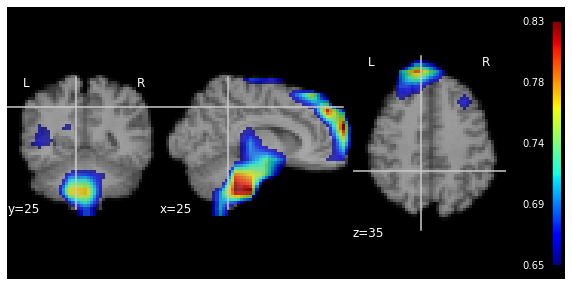
Let's watch the data. We will use nilearn package for the visualisation: https://nilearn.github.io/modules/generated/nilearn.plotting.plot_anat.html#nilearn.plotting.plot_anat

In [4]:

!pip  install --quiet --upgrade nilearn
import nilearn
from nilearn import plotting

     |████████████████████████████████| 9.6 MB 28.1 MB/s 

In [5]:

img = nilearn.image.load_img(data_dir +'100408.nii')
plotting.plot_anat(img)

<nilearn.plotting.displays._slicers.OrthoSlicer at 0x7f723142b4d0>

Questions:

What is the size of image (file)?
That is the intensity distribution of voxels?

In [6]:

img_array = nilearn.image.get_data(img)
img_array.shape

(260, 311, 260)

2. Defining training and target samples

In [7]:

X, y = np.load(data_dir + 'tensors.npy'), \
np.load(data_dir + 'labels.npy')
X = X[:, np.newaxis, :, :, :]
print(X.shape, y.shape)

(1113, 1, 58, 70, 58) (1113,)

In [8]:

sample_data = X[1,0,:,:,:]
X[1,0,:,:,:].shape

(58, 70, 58)

From the sourse article:

The original data were too large to train the model and it would cause RESOURCE EXAUSTED problem while training due to the insufficient of GPU memory. The GPU we used in the experiment is NVIDIAN TITAN_XP with 12G memory each. To solve the problem, we scaled the size of FA image to [58 × 70 × 58]. This procedure may lead to a better classification result, since a smaller size of the input image can provide a larger receptive field to the CNN model. In order to perform the image scaling, “dipy” (http://nipy.org/dipy/) was used to read the .nii data of FA. Then “ndimage” in the SciPy (http://www.scipy.org) was used to reduce the size of the data.

In [9]:

sample_img = nilearn.image.new_img_like(img, sample_data)
plotting.plot_anat(sample_img)

<nilearn.plotting.displays._slicers.OrthoSlicer at 0x7f722e64ca50>

3. Defining Data Set

In [10]:

class MriData(torch.utils.data.Dataset):
    def __init__(self, X, y):
        super(MriData, self).__init__()
        self.X = torch.tensor(X, dtype=torch.float32)
        self.y = torch.tensor(y).long()
    
    def __len__(self):
        return self.X.shape[0]
    
    def __getitem__(self, idx):
        return self.X[idx], self.y[idx]

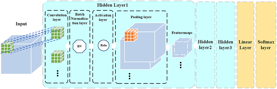
4. Defining the CNN model architecture

3D PCNN architecture model

At first check if we have GPU onborad:

In [11]:

 torch.cuda.is_available()

True

In [12]:

if torch.cuda.is_available():
  device = torch.device("cuda")
else:
  device = torch.device("cpu")

In [13]:

## Hidden layers 1, 2 and 3
hidden = lambda c_in, c_out: nn.Sequential(
    nn.Conv3d(c_in, c_out, (3,3,3)), # Convolutional layer
    nn.BatchNorm3d(c_out), # Batch Normalization layer
    nn.ReLU(), # Activational layer
    nn.MaxPool3d(2) # Pooling layer
)

class MriNet(nn.Module):
    def __init__(self, c):
        super(MriNet, self).__init__()
        self.hidden1 = hidden(1, c)
        self.hidden2 = hidden(c, 2*c)
        self.hidden3 = hidden(2*c, 4*c)
        self.linear = nn.Linear(128*5*7*5, 2)
        self.flatten = nn.Flatten()

    def forward(self, x):
        x = self.hidden1(x)
        x = self.hidden2(x)
        x = self.hidden3(x)
        x = self.flatten(x)
        x = self.linear(x)
        x = F.log_softmax(x, dim=1)
        return x

torch.manual_seed(1)
np.random.seed(1)

c = 32
model = MriNet(c).to(device)
summary(model, (1, 58, 70, 58))

----------------------------------------------------------------
        Layer (type)               Output Shape         Param #
================================================================
            Conv3d-1       [-1, 32, 56, 68, 56]             896
       BatchNorm3d-2       [-1, 32, 56, 68, 56]              64
              ReLU-3       [-1, 32, 56, 68, 56]               0
         MaxPool3d-4       [-1, 32, 28, 34, 28]               0
            Conv3d-5       [-1, 64, 26, 32, 26]          55,360
       BatchNorm3d-6       [-1, 64, 26, 32, 26]             128
              ReLU-7       [-1, 64, 26, 32, 26]               0
         MaxPool3d-8       [-1, 64, 13, 16, 13]               0
            Conv3d-9      [-1, 128, 11, 14, 11]         221,312
      BatchNorm3d-10      [-1, 128, 11, 14, 11]             256
             ReLU-11      [-1, 128, 11, 14, 11]               0
        MaxPool3d-12         [-1, 128, 5, 7, 5]               0
          Flatten-13                [-1, 22400]               0
           Linear-14                    [-1, 2]          44,802
================================================================
Total params: 322,818
Trainable params: 322,818
Non-trainable params: 0
----------------------------------------------------------------
Input size (MB): 0.90
Forward/backward pass size (MB): 201.01
Params size (MB): 1.23
Estimated Total Size (MB): 203.14
----------------------------------------------------------------

5. Training the model

In [14]:

X_train, X_test, y_train, y_test = train_test_split(X, y, test_size=0.2, stratify=y, random_state=42) 
#del X, y #deleting for freeing space on disc

train_dataset = MriData(X_train, y_train)
test_dataset = MriData(X_test, y_test)
#del X_train, X_test, y_train, y_test #deleting for freeing space on disc

In [15]:

train_dataset = MriData(X_train, y_train)
test_dataset = MriData(X_test, y_test)
train_loader = torch.utils.data.DataLoader(train_dataset, batch_size=45, shuffle=True)  #45 - recommended value for batchsize
val_loader = torch.utils.data.DataLoader(test_dataset, batch_size=28, shuffle=False)

In [16]:

CHECKPOINTS_DIR =  data_dir +'/checkpoints'

criterion = nn.NLLLoss().to(device)
optimizer = torch.optim.Adam(model.parameters(), lr=3e-4)
scheduler = torch.optim.lr_scheduler.MultiStepLR(optimizer, milestones=[5, 15], gamma=0.1)

In [17]:

# timing
from tqdm import tqdm

def get_accuracy(net, data_loader):
    net.eval()
    correct = 0
    for data, target in data_loader:
        data = data.to(device)
        target = target.to(device)

        out = net(data)
        pred = out.data.max(1)[1] # get the index of the max log-probability
        correct += pred.eq(target.data).cpu().sum()
        del data, target
    accuracy = 100. * correct / len(data_loader.dataset)
    return accuracy.item()

def get_loss(net, data_loader):
    net.eval()
    loss = 0 
    for data, target in data_loader:
        data = data.to(device)
        target = target.to(device)

        out = net(data)
        loss += criterion(out, target).item()*len(data)

        del data, target, out 

    return loss / len(data_loader.dataset)


def train(epochs, net, criterion, optimizer, train_loader, val_loader, scheduler=None, verbose=True, save=False):
    best_val_loss = 100_000
    best_model = None
    train_loss_list = []
    val_loss_list = []
    train_acc_list = []
    val_acc_list = []

    train_loss_list.append(get_loss(net, train_loader))
    val_loss_list.append(get_loss(net, val_loader))
    train_acc_list.append(get_accuracy(net, train_loader))
    val_acc_list.append(get_accuracy(net, val_loader))
    if verbose:
        print('Epoch {:02d}/{} || Loss:  Train {:.4f} | Validation {:.4f}'.format(0, epochs, train_loss_list[-1], val_loss_list[-1]))

    net.to(device)
    for epoch in tqdm(range(1, epochs+1)):
        net.train()
        for X, y in train_loader:
            # Perform one step of minibatch stochastic gradient descent
            X, y = X.to(device), y.to(device)
            optimizer.zero_grad()
            out = net(X)
            loss = criterion(out, y)
            loss.backward()
            optimizer.step()
            del X, y, out, loss #freeing gpu space
            
        
        # define NN evaluation, i.e. turn off dropouts, batchnorms, etc.
        net.eval()
        for X, y in val_loader:
            # Compute the validation loss
            X, y = X.to(device), y.to(device)
            out = net(X)
            del X, y, out #freeing gpu space
         
        if scheduler is not None:
            scheduler.step()
        
        
        train_loss_list.append(get_loss(net, train_loader))
        val_loss_list.append(get_loss(net, val_loader))
        train_acc_list.append(get_accuracy(net, train_loader))
        val_acc_list.append(get_accuracy(net, val_loader))

        if save and val_loss_list[-1] < best_val_loss:
            torch.save(net.state_dict(), CHECKPOINTS_DIR+'best_model')
        freq = 1
        if verbose and epoch%freq==0:
            print('Epoch {:02d}/{} || Loss:  Train {:.4f} | Validation {:.4f}'.format(epoch, epochs, train_loss_list[-1], val_loss_list[-1]))
        
    return train_loss_list, val_loss_list, train_acc_list, val_acc_list

Training first 20 epochs:

In [ ]:

# training will take ~8 min
torch.manual_seed(1)
np.random.seed(1)
EPOCHS = 20

train_loss_list, val_loss_list, train_acc_list, val_acc_list = train(EPOCHS, model, criterion, optimizer, train_loader, val_loader, scheduler=scheduler, save=False)

Epoch 00/20 || Loss:  Train 45.8454 | Validation 45.9936

  5%|▌         | 1/20 [00:15<05:00, 15.82s/it]

Epoch 01/20 || Loss:  Train 1.7148 | Validation 1.8976

 10%|█         | 2/20 [00:31<04:41, 15.62s/it]

Epoch 02/20 || Loss:  Train 0.3212 | Validation 0.3885

 15%|█▌        | 3/20 [00:46<04:25, 15.63s/it]

Epoch 03/20 || Loss:  Train 0.3118 | Validation 0.4005

 20%|██        | 4/20 [01:02<04:11, 15.72s/it]

Epoch 04/20 || Loss:  Train 0.2400 | Validation 0.2903

 25%|██▌       | 5/20 [01:18<03:56, 15.76s/it]

Epoch 05/20 || Loss:  Train 0.2217 | Validation 0.2894

 30%|███       | 6/20 [01:34<03:39, 15.66s/it]

Epoch 06/20 || Loss:  Train 0.2189 | Validation 0.2849

 35%|███▌      | 7/20 [01:49<03:22, 15.59s/it]

Epoch 07/20 || Loss:  Train 0.2179 | Validation 0.2872

In [ ]:

plt.figure(figsize=(20,8))

plt.subplot(1, 2, 1)
plt.title('Loss history', fontsize=18)
plt.plot(train_loss_list[1:], label='Train')
plt.plot(val_loss_list[1:], label='Validation')
plt.xlabel('# of epoch', fontsize=16)
plt.ylabel('Loss', fontsize=16)
plt.legend(fontsize=16)
plt.grid()

plt.subplot(1, 2, 2)
plt.title('Accuracy history', fontsize=18)
plt.plot(train_acc_list, label='Train')
plt.plot(val_acc_list, label='Validation')
plt.xlabel('# of epoch', fontsize=16)
plt.ylabel('Accuracy', fontsize=16)
plt.legend(fontsize=16)
plt.grid()

K-Fold model validation:

Questions:

What is the purpose of K-Fold in that experiment setting?
Can we afford cross-validation in regular DL?

In [ ]:

# execute for ~ 23 min
skf = StratifiedKFold(n_splits=3, shuffle=True, random_state=42)
cross_vall_acc_list = []
j = 0

for train_index, test_index in skf.split(X, y):
    print('Doing {} split'.format(j))
    j += 1

    X_train, X_test = X[train_index], X[test_index]
    y_train, y_test = y[train_index], y[test_index]
    train_dataset = MriData(X_train, y_train)
    test_dataset = MriData(X_test, y_test)
    train_loader = torch.utils.data.DataLoader(train_dataset, batch_size=45, shuffle=True)  #45 - recommended value for batchsize
    val_loader = torch.utils.data.DataLoader(test_dataset, batch_size=28, shuffle=False) 
    
    torch.manual_seed(1)
    np.random.seed(1)

    c = 32
    model = MriNet(c).to(device)
    criterion = nn.NLLLoss().to(device)
    optimizer = torch.optim.Adam(model.parameters(), lr=3e-4)
    scheduler = torch.optim.lr_scheduler.MultiStepLR(optimizer, milestones=[5, 15], gamma=0.1)

    train(EPOCHS, model, criterion, optimizer, train_loader, val_loader, scheduler=scheduler, save=False, verbose=False) 
    cross_vall_acc_list.append(get_accuracy(model, val_loader))

In [ ]:

print('Average cross-validation accuracy (3-folds):', sum(cross_vall_acc_list)/len(cross_vall_acc_list))

In [ ]:

cross_vall_acc_list

Model save

In [ ]:

# Training model on whole data and saving it
dataset = MriData(X, y)
loader = torch.utils.data.DataLoader(dataset, batch_size=45, shuffle=True)  #45 - recommended value for batchsize

torch.manual_seed(1)
np.random.seed(1)

model = MriNet(c).to(device)
criterion = nn.NLLLoss().to(device)
optimizer = torch.optim.Adam(model.parameters(), lr=3e-4)
scheduler = torch.optim.lr_scheduler.MultiStepLR(optimizer, milestones=[5, 15], gamma=0.1)

train(EPOCHS, model, criterion, optimizer, loader, loader, scheduler=scheduler, save=True, verbose=False) 
pass

What else?

MRI classifcation model interpretation

Visit: https://github.com/kondratevakate/InterpretableNeuroDL

Meaningfull perturbations on MEN brains prediction: