CoCalc News

The LaTeX editor in CoCalc now does rich-text editing directly in the source, without giving up a single character of control over your .tex file.

Your source, rendered in place
Open any .tex file and you'll find a new toolbar with a [ Source | Rich ] toggle. In Rich mode — now the default — CoCalc recognizes standard LaTeX constructs and renders them inline, right where you type:
Math (
$…$,\[…\],equation,align,gather, …) renders with KaTeX, including your own\newcommandmacros from the preamble, so what you see matches what compiles.Text styling —
\textbf,\emph,\underline,\textcolor, font sizes — shows up bold, italic, colored, and sized, with nested commands rendered too.Structure —
\section,\subsection, and lists (itemize/enumerate/description) get a clean visual representation.References & notes —
\ref,\cite,\label,\footnote,\caption, and theorem-like environments (theorem,lemma,proof, …) render as tidy labeled markers.
Anything CoCalc doesn't specifically recognize falls back gracefully: unknown commands become a neutral chip showing the command name, and preamble/config lines simply stay as raw source. Nothing is ever hidden or rewritten behind your back.
Tables
A \begin{tabular}{…} block renders as an actual table. The column specification (l / c / r / p{…}) is honored, and rules — \hline, \toprule, \midrule, \bottomrule, vertical | dividers — show up as real borders. Cell content is rendered too, so inline math like $1 \neq 2$ or a \textbf{…} inside a cell appears formatted rather than as raw source.
This is deliberately fail-open: if a table uses something the renderer can't yet handle cleanly (\multicolumn, \multirow, tabularx, …), CoCalc leaves that block as plain LaTeX source instead of guessing. The toolbar's Table button inserts a ready-to-edit 3×3 tabular to get you started.
Images
\includegraphics{…} renders the actual image inline, pulled from your project's files. A width given as [width=0.5\textwidth] or in absolute units (cm, in, mm, pt, px) is respected, so the preview reflects the size you asked for. If the referenced file can't be found, you get a clear inline placeholder instead of a silent gap — easy to spot a broken path at a glance.
The source is always the truth
This is not a separate WYSIWYG mode that round-trips your document. The CodeMirror buffer remains the one and only canonical source:
Click any widget — or just move your cursor onto that line — and it instantly dissolves back to the raw LaTeX, ready to edit.
Hover a widget to peek at the exact source it represents.
Scroll, edit, and collaborate in real time — widgets reconcile live without flicker, and the rich view stays in sync with whatever you (or a collaborator) type.
Prefer to see everything as plain LaTeX? Flip the toggle to Source and the widgets step aside.
A toolbar that writes LaTeX for you
The new toolbar works in both view modes. Buttons for sections, bold / italic / underline, font size, math, links, lists, verbatim, and a 3×3 table insert the correct LaTeX for you — handy whether you're learning the syntax or just want to move quickly. On narrow panes the controls collapse neatly into a single Format menu.
AI-assisted formulas
Every rendered formula carries a small ✏️ pencil. Click it to open CoCalc's AI formula assistant with the existing equation as context: describe the change in plain language and the formula is rewritten in place, preserving your delimiters. The edit is collaboration-safe — if the surrounding text shifted while the dialog was open, CoCalc declines rather than overwriting the wrong span.
Try it
Open any .tex document in a CoCalc project and start typing — Rich mode is on by default. We'd love your feedback as we expand the set of supported constructs.
Per-region chat threads and collaborative bookmarks now work directly inside LaTeX documents. Drop a short comment on any line and CoCalc attaches a side-chat thread or a named bookmark to that exact location — no sidebar search, no copying line numbers.

Anchored chat threads
Type a LaTeX comment like % chat: review-sec2 (block form on its own line, or inline after content) and a dedicated discussion thread opens for that location. The hash can be a short random ID or a mnemonic of your choice — anything matching [A-Za-z0-9_-]{3,64}.
Gutter icon — every marker line gets a compact chat icon. It turns red when there are unread messages, gray otherwise. Click to open the thread.
Inline tail widget — right after the comment, a pill shows
N unread(red) orN messages(gray), plus a small×to delete the marker with a confirmation.Read-only lock — once a thread has a real message, its anchor line becomes atomic and bold so collaborators don't accidentally renumber or overwrite it. Deleting the root message unlocks the line.
Multi-file — markers work across
\input{...}sub-files. The thread header shows<hash> (file:line)with a Jump button; if the same hash appears in several places, a dropdown lets you pick the destination.Cursor-follow insert — a faint chat icon tracks your cursor in the gutter. Click it to insert a new
% chat:marker on the current line.
Insert a marker from the menu via Insert → Chat or with Ctrl-Shift-M (Shift-Cmd-M on macOS). In split panes, the inserted marker targets the pane you are actually editing.
Collaborative bookmarks
Bookmarks are a lighter cousin of chat anchors — free-form text markers for "remember this spot".
Write
% bookmark: introduction refactoron any line.The Contents panel (Output → Contents) lists bookmarks interleaved with your section hierarchy at a deeper indent, marked with a blue bookmark icon. Clicking jumps to the line.
The gutter shows a gray bookmark icon on each bookmark line.
Insert via Insert → Bookmark or Ctrl-Shift-B (Shift-Cmd-B on macOS). The default text is pre-selected so you can rename it immediately.
Bookmarks don't lock the line and don't create a chat thread — they're purely for navigation and for sharing interesting spots with collaborators.
Why comments?
Because the markers are just LaTeX comments, they travel with the file. They survive copy/paste between projects, show up in git diffs, and are invisible to pdflatex. Open the same .tex file with two users and both see the same icons, threads, and bookmarks in real time.
The same per-region chat model already powers per-cell discussions in Jupyter notebooks; LaTeX now shares that infrastructure, and both benefit from the same fixes — including a small bug where the sender briefly saw their own message as unread.
CoCalc now ships an alternative minimal view for Jupyter notebooks, focused on reading, presenting, and reviewing results. It is the exact same Jupyter notebook underneath — same kernels, same cells, same .ipynb file, fully interchangeable with the classic view — just packaged into a layout that gets code out of the way until you need it.

Side-by-side layout
Outputs live on the left, code on the right. By default the code column fades into the background so your eye lands on results first. Click a code cell to edit and it expands and comes into focus; move away and it fades back. Hover the code column at any time to reveal per-cell run and action buttons — they stay tucked away until you ask for them.
Sectioned notebook
The notebook is automatically divided into sections based on your markdown headings (#, ##, ###, ####). A section's name is the heading text itself — no extra configuration. Each section can be collapsed to hide its cells while you work elsewhere, and executed as a unit with a single click. If you already structure your notebooks with headings, you instantly get a proper outline for navigation and execution.
Mini table of contents
At comfortable and narrow widths a floating TOC appears in the left margin, listing every section heading. Click an entry to jump to that section; double-click to run every code cell in that section. Long notebooks become navigable at a glance, and section-at-a-time iteration is a first-class operation.
Minibar overview
Along the right edge, a compact minibar renders every cell as a small stylized block — a whole-notebook bird's-eye view stacked vertically:
Red blocks mark cells that errored, so broken spots jump out without scrolling.
Green blocks blink while a cell is executing, so you can watch a long run progress.
The currently focused cell is highlighted in blue.
Click or drag to scroll the notebook — the minibar doubles as a tall scroll handle.
In a 200-cell notebook, finding the one cell that blew up turns into a one-glance operation.
Layout widths
Switch between Wide (full width), Comfortable (centered with TOC), and Narrow (compact centered) directly from the status bar. Narrow and comfortable are great for focused reading and presentation; wide maximizes horizontal room for plots and wide DataFrames.
Enhanced run controls
The run button on each cell carries a dropdown with options to run everything above or below — scoped either to the whole notebook or to the current section. Combined with the Mini TOC's double-click-to-run and the section collapse/execute controls, running exactly the right subset of cells is finally simple.
Zen mode
One click hides every code cell, leaving only outputs and markdown. It is the shortest path to a clean reading view for write-ups, presentations, or sharing a notebook with a colleague who just wants the results.
AI Assistant and cell chat
The side-chat AI assistant is wired into the minimal view: ask questions about your code, generate new cells, or debug errors right next to your notebook. Per-cell chat threads show up in the margin as well, with a zen-mode badge so you do not miss unread messages when outputs are all you see.
Frame editor integration
The minimal view is just another frame type, so everything you can do with the classic view still works: split the window, open two frames onto the same notebook, swap a frame for a terminal, or flip back to the classic notebook for full editing. You can mix and match per pane.
Familiar keyboard shortcuts
All the standard Jupyter shortcuts still apply — Shift+Enter to run, Esc/Enter to toggle command and edit mode, arrow keys to navigate. Nothing new to relearn.
Open any .ipynb file and use the frame type toggle to switch between the classic and minimal views. In-app, the status bar has a Help button with a short tour of everything above.
Deeper AI integration, more layout refinements, and better presentation tooling are on the way.
CoCalc now includes a built-in AI Coding Agent: an LLM-powered assistant that lives right inside your editor's side panel.
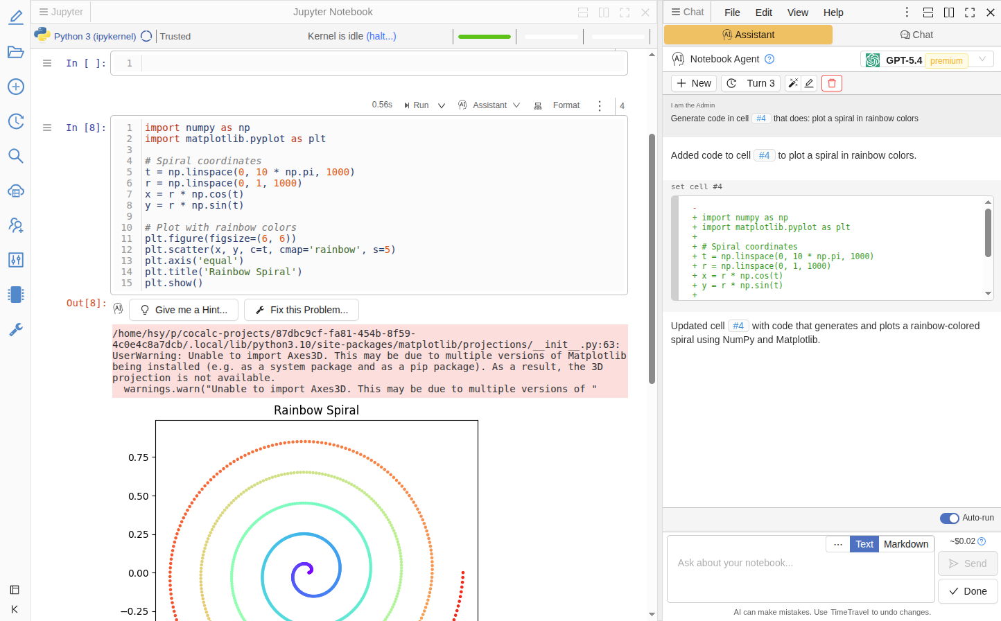
What it does
Instead of just chatting about code, the Coding Agent can directly edit your files. Ask it to fix a bug, refactor a function, or add error handling, and it responds with precise, line-level edits that you review as diffs before applying.
Key features
Works everywhere — Python, R, Julia, JavaScript/TypeScript, C/C++, HTML, Markdown, and many more file types, plus Jupyter notebooks.
Context-aware — The agent sees your cursor position, selected text, and surrounding code. No need to copy-paste context manually.
Safe edits — Either trust it via auto-accepting and revert using TimeTravel, or review all changes.
Shell commands — The agent can suggest terminal commands (install packages, run tests) that you confirm before execution.
Jupyter integration — In notebooks, the agent can create, edit, and run cells. Use the "Generate" button between cells or per-cell tools (Explain, Fix, Modify) to open the agent with context pre-filled.
Session history — Conversations are organized into "turns". You can revisit, rename, or start fresh.
Cost estimation — See estimated token usage before sending each message.
Open the Assistant tab in the side chat panel of any code file or notebook to get started.
LaTeX Agent
Similar to Jupyter and Code, there is also an Assistant tab in a .tex files. It understands LaTeX document structure and applies edits that keep your document valid.
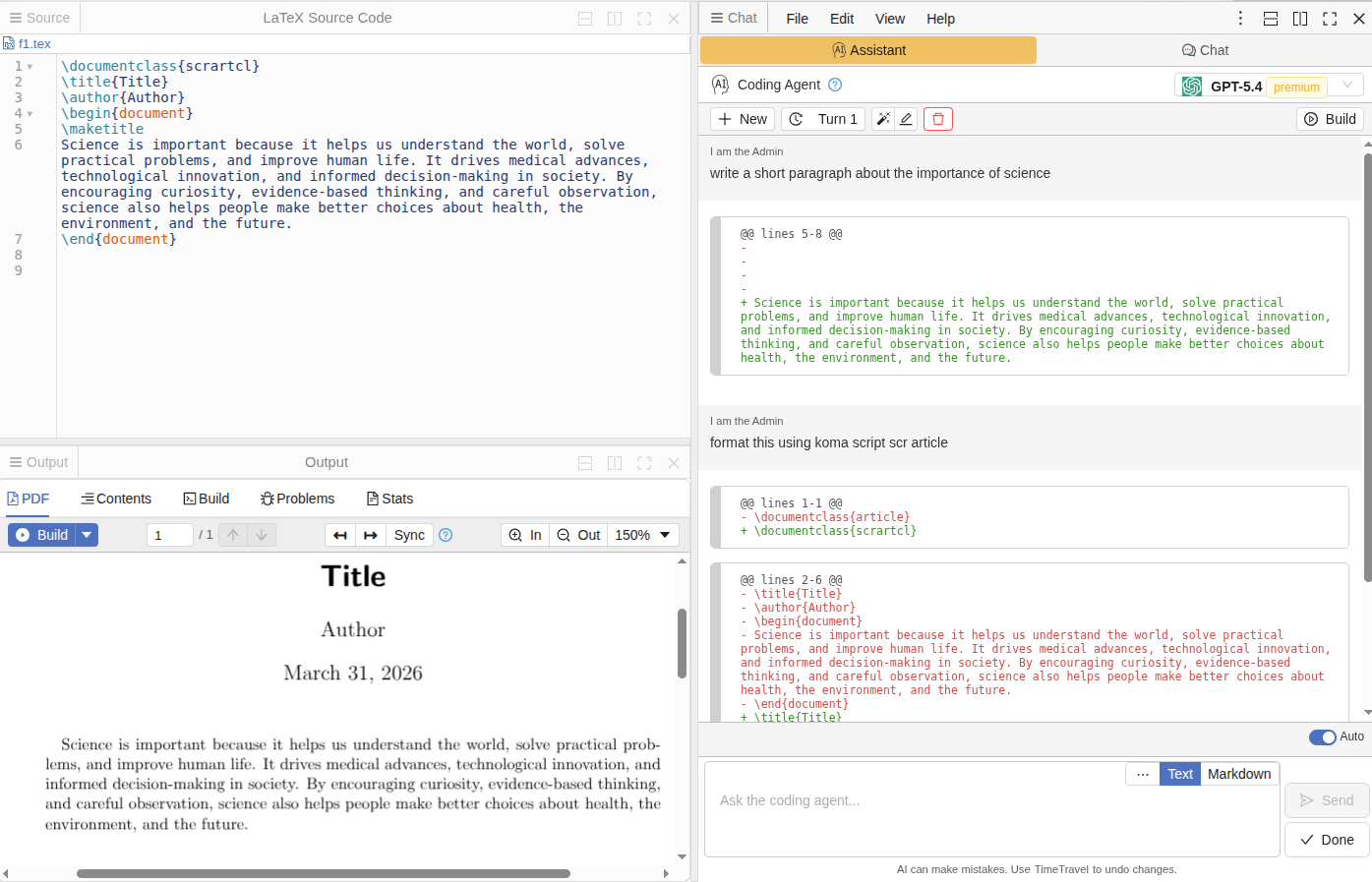
LaTeX-specific capabilities
Environment-aware edits — When a change touches a theorem, proof, align block, or math environment, the agent includes enough surrounding context to ensure the result is syntactically valid.
Minimal but correct — Edits are as small as possible, but never at the cost of leaving broken LaTeX.
Instant error fixing — When a LaTeX build fails, click "Help me fix" in the error gutter — the agent analyzes the error and proposes a fix. Enable auto-accept edits and compilation errors get resolved almost instantly: click, fix, done.
This works alongside CoCalc's existing LaTeX build system, and with enabled auto-build on save, this has the potential to speed up your work with LaTeX significantly.
Open any .tex file and switch to the Assistant tab to try it out.
We just released a software update after quite a lengthy break. It contains updates to basically all the software stacks we offer. If you need to get back to before the update from today, select Ubuntu 24.04 (2025-08-27) in Project Settings → Project Control → Software Environment.
If you're interested in trying out an early single user alpha test version of CoCalc that you can install on your laptop or a server, email us at [email protected], or just try it out [1]. You should expect this to be "alpha quality", etc., but we would be interested in feedback to help with development. The complete source code for this is visible at [3], in case you are curious about how it works.
There will also be very early unstable alpha releases of CoCalc Launchpad at [2], which is a multiuser version of CoCalc, which requires connecting external VM's for running code.
Email [email protected] and asked to be added to the official alpha testers group if you want more details, guidance, and to provide feedback.
[1] https://software.cocalc.ai/software/cocalc-plus/index.html
[2] https://software.cocalc.ai/software/cocalc-launchpad/index.html
CoCalc now has an update API client with preliminary support for connecting to an MCP server. After you installed the cocalc-api from source and configured the MCP server you can talk to your projects.
Here is a simple demo example:

Which indeed modified a file in my project:

I made a first ever early alpha release of Cocalc+! It's here: https://github.com/sagemathinc/cocalc/releases/tag/0.2.5
What is this? It's a locally installable version of CoCalc that does NOT require Docker, and lets you fully use whatever Jupyter kernels, latex, etc. you have on your own laptop directly. It's a single self-contained binary, and is very lightweight.
Try it, with the caveats of course that it's probably horribly broken.
There is an Apple Silicon mac binary that is properly signed.
There's a Linux binary for x86_64 as well.
Most importantly, this is the first version of CocalcPlus ever that actually has AI support, which was a significant amount of work to add. To configure AI, click on the settings icon in the UPPER RIGHT, then click on "AI" and paste in a key and click save. You might need to refresh your browser, but you'll get full AI integration for the provides you configure.
You can also run this on a remote server and thus use the CoCalc UI, TimeTravel, Jupyter notebooks, whiteboards, latex editor, terminals, etc., and thus more easily use that remote server.
The design is very lightweight in that it is single user and there is only one project -- your computer. There is also no separate database.
This does not currently support integration with cocalc.com, but that is of course planned soon as an option. The model is that CoCalc+ will be free, but some integrations with our cloud services will require a subscription.
I developed a brand new Python api for using CoCalc!
https://pypi.org/project/cocalc-api/
and you should be able to pip or uv install it as normal.
The docs are at
https://cocalc.com/api/python/
You might want to try a few basic things like:
create an api key in account prefs on cocalc (refresh your browser if you get an error setting the expire date, since I just fixed an issue)
use the api to list your projects,
create a project,
copy files between two projects
Organizations
CoCalc now has a notion of organizations with admins, who can manage users of an organization. This is currently only accessible via this Python API right now. It is designed to make it much easier to build things like asynchronous courses involving Jupyter notebooks, where you want to easily build your own custom workflow and user management instead of using CoCalc's course management UI.
For managing users we will need to create a new "organization" for you and make you an admin of that organization. You can then create users in your org, provide a URL so they can use cocalc (without having to worry about creating accounts themselves), etc. Can you also make projects for them, add them as collaborators to those projects, copy files to their projects (from your own template project), list all members of your org, etc. It's also easy to broadcast a message to all org members.
It's also fairly easy to add new functionality to this API. What is missing that you want? An obvious gap is compute servers, right now.
-- William
Starting today, our default software environment for new projects is based on Ubuntu 24.04. You can still select the previous default, Ubuntu 22.04 (available until June 2025), when creating new projects. While we plan to support Ubuntu 22.04 for a while longer, our main focus going forward will be on Ubuntu 24.04.
Existing projects are unaffected. If you want to switch, you can do this any time via Project Settings → Project Control → Software Environment.
To see what’s included, check out our software inventory.
Programming Languages and Features
Python: There is now a new "CoCalc Python" environment, featuring a curated set of popular packages. This replaces the previously called "system-wide" environment. Terminals now run inside this environment by default. The main benefit is, that this allows to manage Python packages without depending on system-wide packages, installed for system utilities. As before, you can also use the Anaconda-based environment via
anaconda2025, and we continue to offer a Colab-compatible environment.R: We now provide a broader selection of R packages, powered by r2u, making it easier and more convenient to get started.
SageMath: The latest version of SageMath is available in the new environment. For earlier SageMath releases, please switch to the "Ubuntu 22.04" environment.
LaTeX: This is now running a full and up-to-date Texlive distribution. We plan to update its packages with each new software environment update.