CoCalc Logo Icon
StoreFeaturesDocsShareSupportNewsAboutSign UpSign In
adasegroup

CoCalc provides the best real-time collaborative environment for Jupyter Notebooks, LaTeX documents, and SageMath, scalable from individual users to large groups and classes!

GitHub Repository: adasegroup/NEUROML2022
Path: blob/main/seminar4/GroupAnalysis.ipynb
Views: 63
Kernel: Python 3

Group Analysis

We often want to generalize the results from our experiment to out of sample data. Here we will infer from the individual subjects activation maps to one activation map for all subjects.

To do this the following steps must be done:

1. Normalize the subjects data to a common space

2. Build a second level GLM

3. Hypothesis testing

Group Analysis

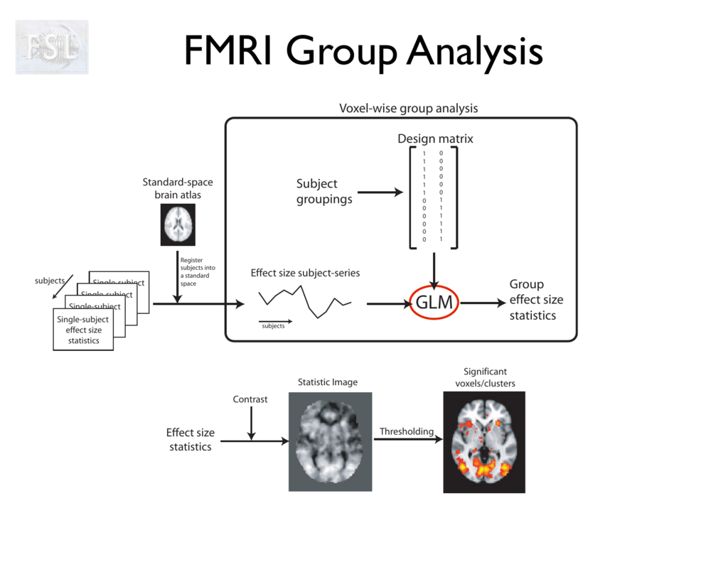
The second level GLM has the form β=βgXg+η {\beta}= {\beta}_g X_g + {\eta}

where:

XgX_g - new design matrix

β{\beta} - estimated from 1st level

Then we can find βg{\beta}_g and perform hypothesis testing on it

Normalize data to MNI template

We will take the computed 1st-level contrasts from the previous experiment and normalize them into MNI-space.

Preparation

We first need to download the already computed deformation field.

%%bash datalad get -J 4 -d /data/ds000114 /data/ds000114/derivatives/fmriprep/sub-0[2345789]/anat/*h5

Alternatively: Prepare yourself

We're using the precomputed warp field from fmriprep, as this step otherwise would take up too much time. If you're nonetheless interested in computing the warp parameters with ANTs yourself, without using fmriprep, either check out the script ANTS_registration.py or even quicker, use RegistrationSynQuick, Nipype's implementation of antsRegistrationSynQuick.sh.

Normalization with ANTs

The normalization with ANTs requires that you first compute the transformation matrix that would bring the anatomical images of each subject into template space. Depending on your system this might take a few hours per subject. To facilitate this step, the transformation matrix is already computed for the T1 images.

The data for it can be found under:

!ls /data/ds000114/derivatives/fmriprep/sub-*/anat/*h5

Now, let's start with the ANTs normalization workflow!

Imports

First, we need to import all the modules we later want to use.

from os.path import join as opj from nipype import Workflow, Node, MapNode from nipype.interfaces.ants import ApplyTransforms from nipype.interfaces.utility import IdentityInterface from nipype.interfaces.io import SelectFiles, DataSink from nipype.interfaces.fsl import Info from nilearn import plotting %matplotlib inline from nipype.interfaces.spm import (OneSampleTTestDesign, EstimateModel, EstimateContrast, Threshold) from nipype.algorithms.misc import Gunzip

Experiment parameters

We will run the group analysis without subject sub-01, sub-06 and sub-10 because they are left-handed.

This is because all subjects were asked to use their dominant hand, either right or left. There were three subjects (sub-01, sub-06 and sub-10) that were left-handed.

Because of this, We will use only right-handed subjects for the following anlysis.

experiment_dir = '/output' output_dir = 'datasink' working_dir = 'workingdir' # list of subject identifiers (remember we use only right handed subjects) subject_list = ['02', '03', '04', '05', '07', '08', '09'] # task name task_name = "fingerfootlips" number_contrasts = 5 # number of contrast from 1stlevel # Template to normalize to template = '/data/ds000114/derivatives/fmriprep/mni_icbm152_nlin_asym_09c/1mm_T1.nii.gz'

Specify Nodes

Initiate ANTs interface

# Apply Transformation - applies the normalization matrix to contrast images apply2con = MapNode(ApplyTransforms(args='--float', input_image_type=3, interpolation='BSpline', invert_transform_flags=[False], num_threads=1, reference_image=template, terminal_output='file'), name='apply2con', iterfield=['input_image'])

Specify input & output stream

Specify where the input data can be found & where and how to save the output data.

# Infosource - a function free node to iterate over the list of subject names infosource = Node(IdentityInterface(fields=['subject_id']), name="infosource") infosource.iterables = [('subject_id', subject_list)] # SelectFiles - to grab the data (alternativ to DataGrabber) templates = {'con': opj(output_dir, '1stLevel', 'sub-{subject_id}/', '???_00??.nii'), 'transform': opj('/data/ds000114/derivatives/fmriprep/', 'sub-{subject_id}', 'anat', 'sub-{subject_id}_t1w_space-mni152nlin2009casym_warp.h5')} selectfiles = Node(SelectFiles(templates, base_directory=experiment_dir, sort_filelist=True), name="selectfiles") # Datasink - creates output folder for important outputs datasink = Node(DataSink(base_directory=experiment_dir, container=output_dir), name="datasink") # Use the following DataSink output substitutions substitutions = [('_subject_id_', 'sub-')] subjFolders = [('_apply2con%s/' % (i), '') for i in range(number_contrasts)] substitutions.extend(subjFolders) datasink.inputs.substitutions = substitutions

Specify Workflow (ANTs)

Create a workflow and connect the interface nodes and the I/O stream to each other.

# Initiation of the ANTs normalization workflow antsflow = Workflow(name='antsflow') antsflow.base_dir = opj(experiment_dir, working_dir) # Connect up the ANTs normalization components antsflow.connect([(infosource, selectfiles, [('subject_id', 'subject_id')]), (selectfiles, apply2con, [('con', 'input_image'), ('transform', 'transforms')]), (apply2con, datasink, [('output_image', 'norm_ants.@con')]), ])

Visualize the workflow

# Create ANTs normalization graph antsflow.write_graph(graph2use='colored', format='png', simple_form=True) # Visualize the graph from IPython.display import Image Image(filename=opj(antsflow.base_dir, 'antsflow', 'graph.png'))

Run the Workflow

Now that everything is ready, we can run the ANTs normalization workflow.

antsflow.run('MultiProc')

Visualize Results

from nilearn.plotting import plot_stat_map %matplotlib inline subject_id = '02' anatimg = '/data/ds000114/derivatives/fmriprep/mni_icbm152_nlin_asym_09c/1mm_T1.nii.gz'

First, let's chek the normalization of anatomical image:

plot_stat_map( f'/data/ds000114/derivatives/fmriprep/sub-{subject_id}/anat/sub-{subject_id}_t1w_space-mni152nlin2009casym_preproc.nii.gz', title='anatomy - ANTs (normalized to ICBM152)', bg_img=anatimg, threshold=200, display_mode='ortho', cut_coords=(-50, 0, -10))

And what about the contrast images for Foot > others?

plot_stat_map( f'/output/datasink/norm_ants/sub-{subject_id}/con_0005_trans.nii', title='Foot > others - Normed', bg_img=anatimg, threshold=2, vmax=5, display_mode='ortho', cut_coords=(-39, -37, 56))
from nilearn.plotting import plot_glass_brain plot_glass_brain( f'/output/datasink/norm_ants/sub-{subject_id}/con_0005_trans.nii', colorbar=True, threshold=3, display_mode='lyrz', black_bg=True, vmax=6, title='contrast5 - ANTs')

2nd level analysis

After we normalized the subjects data into template space, we can now do the group analysis.

experiment_dir = '/output' output_dir = 'datasink' working_dir = 'workingdir' # Which contrasts to use for the 2nd-level analysis contrast_list = ['con_0001', 'con_0002', 'con_0003', 'con_0004', 'con_0005'] mask = "/data/ds000114/derivatives/fmriprep/mni_icbm152_nlin_asym_09c/1mm_brainmask.nii.gz"
!tree /output/datasink/2ndLevel
# Gunzip - unzip the mask image gunzip = Node(Gunzip(in_file=mask), name="gunzip") # OneSampleTTestDesign - creates one sample T-Test Design onesamplettestdes = Node(OneSampleTTestDesign(), name="onesampttestdes") # EstimateModel - estimates the model level2estimate = Node(EstimateModel(estimation_method={'Classical': 1}), name="level2estimate") # EstimateContrast - estimates group contrast level2conestimate = Node(EstimateContrast(group_contrast=True), name="level2conestimate") cont1 = ['Group', 'T', ['mean'], [1]] level2conestimate.inputs.contrasts = [cont1] # Threshold - thresholds contrasts, we use fdr correction level2thresh = Node(Threshold(contrast_index=1, use_topo_fdr=True, use_fwe_correction=False, extent_threshold=0, height_threshold=0.005, height_threshold_type='p-value', extent_fdr_p_threshold=0.05), name="level2thresh") # Infosource - a function free node to iterate over the list of subject names infosource = Node(IdentityInterface(fields=['contrast_id']), name="infosource") infosource.iterables = [('contrast_id', contrast_list)] # SelectFiles - to grab the data templates = {'cons': opj(output_dir, 'norm_ants', 'sub-*', '{contrast_id}_trans.nii')} selectfiles = Node(SelectFiles(templates, base_directory=experiment_dir, sort_filelist=True), name="selectfiles") # Datasink - creates output folder for important outputs datasink = Node(DataSink(base_directory=experiment_dir, container=output_dir), name="datasink") # Use the following DataSink output substitutions substitutions = [('_contrast_id_', '')] datasink.inputs.substitutions = substitutions
# Initiation of the 2nd-level analysis workflow l2analysis = Workflow(name='ants_l2analysis') l2analysis.base_dir = opj(experiment_dir, working_dir) # Connect up the 2nd-level analysis components l2analysis.connect([(infosource, selectfiles, [('contrast_id', 'contrast_id')]), (selectfiles, onesamplettestdes, [('cons', 'in_files')]), (gunzip, onesamplettestdes, [('out_file', 'explicit_mask_file')]), (onesamplettestdes, level2estimate, [('spm_mat_file', 'spm_mat_file')]), (level2estimate, level2conestimate, [('spm_mat_file', 'spm_mat_file'), ('beta_images', 'beta_images'), ('residual_image', 'residual_image')]), (level2conestimate, level2thresh, [('spm_mat_file', 'spm_mat_file'), ('spmT_images', 'stat_image'), ]), (level2conestimate, datasink, [('spm_mat_file', '2ndLevel.@spm_mat'), ('spmT_images', '2ndLevel.@T'), ('con_images', '2ndLevel.@con')]), (level2thresh, datasink, [('thresholded_map', '2ndLevel.@threshold')]), ])
l2analysis.write_graph(graph2use='flat', format='png', simple_form=True) Image(filename='/output/workingdir/ants_l2analysis/graph_detailed.png')
l2analysis.run('MultiProc', plugin_args={'n_procs': 4})
#!nipypecli crash /home/neuro/nipype_tutorial/lection/crash-20200721-181746-neuro-selectfiles.a5-607b7489-d773-4d9c-ae69-49eca16a30d1.pklz

Keep in mind, that the group analysis was only done on N=7 subjects, and that we chose a voxel-wise threshold of p<0.005. Nonetheless, we corrected for multiple comparisons with a cluster-wise FDR threshold of p<0.05.

So let's first look at the contrast average:

Let's take a look at the files we produced

!tree /output/datasink/2ndLevel
anatimg = '/data/ds000114/derivatives/fmriprep/mni_icbm152_nlin_asym_09c/1mm_T1.nii.gz' plot_stat_map( '/output/datasink/2ndLevel/con_0001/spmT_0001_thr.nii', title='ants', dim=1, bg_img=anatimg, threshold=2, vmax=8, display_mode='y', cut_coords=(-45, -30, -15, 0, 15), cmap='viridis');

Now, let's see other contrast Foot > others using the glass brain plotting method.

from nilearn.plotting import plot_glass_brain plot_glass_brain( '/output/datasink/2ndLevel/con_0005/spmT_0001_thr.nii', colorbar=True, threshold=2, display_mode='lyrz', black_bg=True, vmax=10, title='Foot > others');

Multiple comparison problem

When we make statistical maps we set a threshold at a given confidence level α\alpha and declare all voxels for which beta is above this this level as active. Typically our H0H_0 is that the voxel is not active.

Hypothesis testing

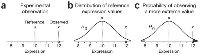
The probability that a test will correctly reject H0H_0 is called the power of the test.

During fMRI experiments we perform test for each voxel, which means there will be many false active voxels. There are many ways to deal with this problem.

How to choose the threshold ?

for tr in [2, 4, 5, 7]: plot_stat_map( '/output/datasink/2ndLevel/con_0001/spmT_0001.nii', title=f'threshold {tr}', dim=1, bg_img=anatimg, threshold=tr, vmax=8, display_mode='y', cut_coords=(-45, -30, -15, 0, 15), cmap='viridis');

FWER (family-wize error rate) methods

We control for any false positives FPFP: FWER=P(FP1)FWER=P(FP \geq 1) H0H_0 is that there is no activation in any of the VV voxels.

Control for type 1 errors(We wrongly have rejected the H0H_0).

Bonferoni correction. The threshold is adjusted as α/V\alpha/V.

Decreases too much the probability of correctly rejecting H0H_0.

The voxels are not completely independent.

Random field theory estimates the number of independent statistical tests based upon the spatial correlation, or smoothness.

The number of independent comparisons for smoothed data is: V/FWHM3V /FWHM^3

where FWHMFWHM-full width at half maximum

At a smoothness of 3 voxels, there would be 1 /27 as many independent comparisons.

The Euler characteristic of the data give us estimation how many clusters of activity should be found by chance at a given statistical threshold

FWER methods often give too conservative threshold, oftentimes FDR gives a better threshold.

FDR (False discovery rate)

Control for the false positives FPFP among all declared positives PP. FDR=E(FP/P)FDR=E(FP/P)

Let's take a look how the popular Benjamini and Hochberg FDR procedure work.

import numpy as np np.random.seed(1) #define a treshold level level = 0.05 #here we simulate some data to work with #how the treshold is affected by changing signal_to_noise? n_points = 2000 signal_to_noise = 0.5 noise = np.random.uniform(size=int(n_points*(1-signal_to_noise))) #signal = np.random.uniform(size=int(n_points*signal_to_noise), high=0.001) signal = np.random.beta(a=0.1,b=8, size=int(n_points*signal_to_noise)) pvals = np.concatenate([noise, signal]) #rank and sort the p values pvals_sortind = np.argsort(pvals) pvals_sorted = pvals[pvals_sortind] n_samples = pvals.shape[0] # the active points are the ones with: p_valule < (rank/n_samples)*level above_tresh = (np.arange(1,n_samples+1)*level/n_samples>pvals_sorted) positive = np.cumsum(above_tresh[::-1])[::-1] #declare positive all points with rank less then the last postive #Let't plot the result import matplotlib.pyplot as plt cols = ['red' if p else 'green' for p in positive] fig, ax = plt.subplots(figsize=(14,6)) ax.scatter(range(n_samples), pvals_sorted, c=cols, marker='.') ax.set_xlabel('ranks') ax.set_ylabel('p values') #lets add Bonferoni treshold for comparison ax.plot([0, n_samples],[0, level], label='BH treshold')#Benjamini and Hochberg plt.axhline(y=level/n_samples, color='black', ls='dashed', alpha = 0.5, label='Bonferoni treshold') _ = ax.legend()
import nibabel data = np.array(nibabel.load('/output/datasink/2ndLevel/con_0001/spmT_0001.nii').dataobj).flatten() plt.hist(data, bins=100) plt.gca().set_ylim([0, 200000])

Special thanks to Michael Notter for the wonderful nipype tutorial