CoCalc Logo Icon
StoreFeaturesDocsShareSupportNewsAboutSign UpSign In
adasegroup

CoCalc provides the best real-time collaborative environment for Jupyter Notebooks, LaTeX documents, and SageMath, scalable from individual users to large groups and classes!

GitHub Repository: adasegroup/NEUROML2022
Path: blob/main/seminar4/IndividualAnalysis.ipynb
Views: 63
Kernel: Python 3

GLM: 1st-level Analysis

The objective in this example is to model the timecourse of each voxel. This will allow us to answer question regarding to the voxel response to different stimuli.

We will model the activation at each voxel yy as a weighed sum of explanatory variables xix_{i} and error term ϵ{\epsilon}

y=β0+i=1Nxiβi+ϵ{y} = {\beta}_{0} + \sum \limits _{i=1} ^{N} x_{i}{\beta}_{i} + {\epsilon}

or in matrix notation

y=βX+ϵy = {\beta} X + {\epsilon}

which can be solved with Ordinary Least Squares regression.

The parameters β{\beta} represent the contribution of each variable to the voxel activation.

The error terms are assumed to be independent and identically distributed.

Design matrix

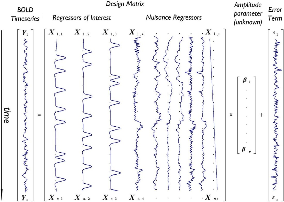
The matrix 𝑋 is also called design matrix.It is up to the researcher which factors to include in the design matrix. The design matrix contains factors that a related to the hypothesis the researcher want to answer. Furthermore, sometimes in it are also included factors that are not related to the hypothesis, but are know sources of variability (nuisance factors).

Now lets take a look how we take into account the delayed bold response. The hemodynamic response function might look something like this:

import numpy as np import matplotlib.pyplot as plt def hrf(t): return t ** 8.6 * np.exp(-t / 0.547) hrf_times = np.arange(0, 20, 0.1) hrf_signal = hrf(hrf_times) plt.plot(hrf_times, hrf_signal) plt.xlabel('time') plt.ylabel('BOLD signal') _ = plt.title('HRF')

In the design often we want to include variables, that indicate presence or absence of a stimuli. Let's say we had the 3 stimuli during the timecourse

n_time_points = 40 times = np.arange(0, n_time_points) neural_signal = np.zeros(n_time_points) neural_signal[4:6] = 1 # A 3 second event neural_signal[9:11] = 1 neural_signal[22:24] = 1 plt.plot(times, neural_signal) plt.xlabel('time (seconds)') plt.ylabel('neural signal') plt.ylim(0, 3.2) _ = plt.title('Neural model for three impulses')

Next we have to convolve signal with our hrf function

hrf_times = np.arange(20) hrf_signal = hrf(hrf_times) bold_signal = np.convolve(neural_signal, hrf_signal) tailed_respose_times = np.arange(n_time_points + hrf_times.shape[0] - 1) plt.plot(tailed_respose_times, bold_signal) plt.xlabel('time (seconds)') plt.ylabel('bold signal') _ = plt.title('Convolved signals')

After that we can fit our fMRI data to the design Matrix and use GLM to for hypotesis testing. We can evaluate whether a given factor ii has a considerable contribution by its coefficient βi{\beta}_{i}. With t-test we can evaluate whether βi{\beta}_{i} > 0. We can also test hypothesis of the form βi{\beta}_{i} > βj{\beta}_{j}.

The general form of the hypothesis tests which forms a contrast is: i=1Pciβi>0\sum \limits _{i=1} ^{P} c_{i}{\beta}_{i} > 0

Typical values for cc are 1 and -1. Typically contrasts are express as:[c1,c2,...,cN] [c_{1}, c_{2}, ..., c_{N}].

For example the contrast [1, 0] tests β1{\beta}_{1} > 0.

This contrasts form a t-statistics (Recall that coefficient/std(coefficient) in OLS regression follow t-distribution with n-p-1 df).

We can combine several contrasts and form F-statics. In the contexts of fMRI the F-tests help us answer questions like "Is effect A or effect B or effect C, or any combination of them, significantly non-zero?".

Recall that F test is used for comparison between reduced model RF and full model FM: F=(SSE(RM)SSR(FM))/(p+1k))SSE(FM)/(np1) F = \frac{(SSE(RM)-SSR(FM)) /(p+1-k))}{SSE(FM)/(n-p-1)}

where the reduced model have k distinct parameters

Combining the test results from all voxels we get statistical map of brain activity. Now that the theory out of our way we can see how it is done in Nipype.

1st Leval Analysis in Nipype

We will use the preprocessed files we got and run 1st-level analysis (individual analysis) for each subject. We will perform the following steps:

  1. Extract onset times of stimuli from TVA file

  2. Specify the model (TR, high pass filter, onset times, etc.)

  3. Specify contrasts to compute

  4. Estimate contrasts

import pandas as pd import os from nilearn import plotting %matplotlib inline from nipype.interfaces.spm import Level1Design, EstimateModel, EstimateContrast from nipype.algorithms.modelgen import SpecifySPMModel from nipype.interfaces.utility import Function, IdentityInterface from nipype.interfaces.io import SelectFiles, DataSink from nipype import Workflow, Node from utils import list_files
# specify paths experiment_dir = '/output' output_dir = 'datasink' working_dir = 'workingdir' # list of subject identifiers subject_list = ['01', '02', '03', '04', '05', '06', '07', '08', '09', '10'] #subject_list = ['01', '02'] # Repetition time(TR) of functional images TR = 2.5

Prepare design matrix

Let's take a look how the stimuli onset and duration look like.This information is store in a tsv file. This file will help us build the design matrix.

The three different conditions in the fingerfootlips task are:

  • finger

  • foot

  • lips

trialinfo = pd.read_table('/data/ds000114/task-fingerfootlips_events.tsv') trialinfo.head()
def subjectinfo(subject_id): import pandas as pd from nipype.interfaces.base import Bunch trialinfo = pd.read_table('/data/ds000114/task-fingerfootlips_events.tsv') #trialinfo.head() conditions = [] onsets = [] durations = [] for group in trialinfo.groupby('trial_type'): conditions.append(group[0]) onsets.append(list(group[1].onset - 10)) # subtracting 10s due to removing of 4 dummy scans durations.append(group[1].duration.tolist()) subject_info = [Bunch(conditions=conditions, onsets=onsets, durations=durations )] return subject_info # this output will later be returned to infosource # Get Subject Info - get subject specific condition information getsubjectinfo = Node(Function(input_names=['subject_id'], output_names=['subject_info'], function=subjectinfo), name='getsubjectinfo')

Initiate Nodes

# SpecifyModel - Generates SPM-specific Model #Setup #https://nipype.readthedocs.io/en/latest/api/generated/nipype.algorithms.modelgen.html#specifymodel modelspec = Node(SpecifySPMModel(concatenate_runs=False, input_units='secs', output_units='secs', time_repetition=TR, high_pass_filter_cutoff=128), name="modelspec") # Level1Design - Generates an SPM design matrix #https://www.fil.ion.ucl.ac.uk/spm/doc/manual.pdf#page=59 #hrf- Name of basis function(canonical) #'derivs': [1, 0]-Time derivatives : Time and Dispersion #model_serial_correlations-serial correlations using an autoregressive estimator (order 1) level1design = Node(Level1Design(bases={'hrf': {'derivs': [1, 0]}}, timing_units='secs', interscan_interval=TR, model_serial_correlations='AR(1)'), name="level1design") # EstimateModel - estimate the parameters of the model #https://www.fil.ion.ucl.ac.uk/spm/doc/manual.pdf#page=69 level1estimate = Node(EstimateModel(estimation_method={'Classical': 1}), name="level1estimate") # EstimateContrast - estimates contrasts level1conest = Node(EstimateContrast(), name="level1conest")

Specify contrasts

We are gona perform several T tests and one F test. Recall the general form of the hypothesis are

i=1Nciβi>0\sum \limits _{i=1} ^{N} c_{i}{\beta}_{i} > 0
# Condition names condition_names = ['Finger', 'Foot', 'Lips'] # Contrasts # contrast = [<contrast_name>, <test>, <condition_names>, <[c1, c2, c3]>] cont01 = ['average', 'T', condition_names, [1/3., 1/3., 1/3.]] cont02 = ['Finger', 'T', condition_names, [1, 0, 0]] cont03 = ['Foot', 'T', condition_names, [0, 1, 0]] cont04 = ['Lips', 'T', condition_names, [0, 0, 1]] cont05 = ['Foot > others', 'T', condition_names, [-0.5, 1, -0.5]] cont06 = ['activation', 'F', [cont02, cont03, cont04]] contrast_list = [cont01, cont02, cont03, cont04, cont05, cont06]

Specify input & output stream

Specify where the input data can be found & where and how to save the output data.

#Infosource - a function free node to iterate over the list of subject names infosource = Node(IdentityInterface(fields=['subject_id', 'contrasts'], contrasts=contrast_list), name="infosource") infosource.iterables = [('subject_id', subject_list)] # SelectFiles - to grab the data (alternativ to DataGrabber) templates = { 'func': 'datasink/preproc/sub-{subject_id}/task-{task_id}/fwhm-5_ssub-{subject_id}_ses-test_task-{task_id}_bold.nii', 'mc_param': 'datasink/preproc/sub-{subject_id}/task-{task_id}/sub-{subject_id}_ses-test_task-{task_id}_bold.par', 'outliers': 'datasink/preproc/sub-{subject_id}/task-{task_id}/art.sub-{subject_id}_ses-test_task-{task_id}_bold_outliers.txt' } selectfiles = Node(SelectFiles(templates, base_directory=experiment_dir, sort_filelist=True), name="selectfiles") selectfiles.inputs.task_id = 'fingerfootlips' # Datasink - creates output folder for important outputs datasink = Node(DataSink(base_directory=experiment_dir, container=output_dir), name="datasink") # Use the following DataSink output substitutions substitutions = [('_subject_id_', 'sub-')] datasink.inputs.substitutions = substitutions

Specify Workflow

Create a workflow and connect the interface nodes and the I/O stream to each other.

# Initiation of the 1st-level analysis workflow l1analysis = Workflow(name='l1analysis') l1analysis.base_dir = f'{experiment_dir}/{working_dir}' # Connect up the 1st-level analysis components l1analysis.connect([(infosource, selectfiles, [('subject_id', 'subject_id')]), (infosource, getsubjectinfo, [('subject_id', 'subject_id')]), (getsubjectinfo, modelspec, [('subject_info', 'subject_info')]), (infosource, level1conest, [('contrasts', 'contrasts')]), (selectfiles, modelspec, [('func', 'functional_runs')]), (selectfiles, modelspec, [('mc_param', 'realignment_parameters'), ('outliers', 'outlier_files')]), (modelspec, level1design, [('session_info', 'session_info')]), (level1design, level1estimate, [('spm_mat_file', 'spm_mat_file')]), (level1estimate, level1conest, [('spm_mat_file', 'spm_mat_file'), ('beta_images', 'beta_images'), ('residual_image', 'residual_image')]), (level1conest, datasink, [('spm_mat_file', '1stLevel.@spm_mat'), ('spmT_images', '1stLevel.@T'), ('con_images', '1stLevel.@con'), ('spmF_images', '1stLevel.@F'), ('ess_images', '1stLevel.@ess'), ]), ])

Visualize the workflow

# Save the 1st-level analysis graph as png l1analysis.write_graph(graph2use='colored', format='png', simple_form=True) # Visualize the graph from IPython.display import Image Image(filename=f'{l1analysis.base_dir}/l1analysis/graph.png')
# show detailed workflow l1analysis.write_graph(graph2use='flat', format='png', simple_form=True) Image(filename=f'{l1analysis.base_dir}/l1analysis/graph_detailed.png')

Run the Workflow

Run the 1st-level analysis workflow.

Run with 'Linear' plugin if multiprocessing frozen during execution

l1analysis.run('MultiProc')
l1analysis.run('Linear')
#Crashs information is stored in .pklz files # In case of a crash use the following command #!nipypecli crash <Last generated .pklz file>

Inspect output

Let's check the structure of the output folder, to see if we have everything we wanted to save. You should one image for each subject and contrast (con_*.nii for T-contrasts and ess_*.nii for F-contrasts)

!tree /output/datasink/1stLevel

Visualize results

Let's look at the contrasts of one subject that we've just computed.

from nilearn.plotting import plot_stat_map #Reminder the tests were test_to_number = { 1: 'average', 2: 'Finger', 3: 'Foot', 4: 'Lips', 5: 'Foot > others', 6: 'activation' } subject_id = '01' anatimg = f'/data/ds000114/derivatives/fmriprep/sub-{subject_id}/anat/sub-{subject_id}_t1w_preproc.nii.gz'
subject_id = '01' anatimg = f'/data/ds000114/derivatives/fmriprep/sub-{subject_id}/anat/sub-{subject_id}_t1w_preproc.nii.gz' for contrast_id in range(1, 6): plot_stat_map( f'/output/datasink/1stLevel/sub-{subject_id}/spmT_000{contrast_id}.nii', title=test_to_number[contrast_id], bg_img=anatimg, threshold=3, display_mode='y', cut_coords=(-5, 0, 5, 10, 15), dim=-1);
contrast_id = 6 subject_id = '01' plot_stat_map( f'/output/datasink/1stLevel/sub-{subject_id}/spmF_000{contrast_id}.nii', title=test_to_number[contrast_id], bg_img=anatimg, threshold=3, display_mode='y', cut_coords=(-5, 0, 5, 10, 15), dim=-1);